
Algorithms and methods of unconstrained optimization. Classical methods of unconstrained optimization. Expert assessment methods
The most acceptable version of the decision that is made at the management level regarding any issue is considered to be optimal, and the process of its search itself is considered optimization.
The interdependence and complexity of organizational, socio-economic, technical and other aspects of production management currently boils down to making a management decision, which affects a large number of different kinds of factors closely intertwined with each other, which makes it impossible to analyze each separately using traditional analytical methods.
Most of the factors are decisive in the decision-making process, and they (in their essence) do not lend themselves to any quantitative characterization. There are also those that are practically unchanged. In this regard, it became necessary to develop special methods capable of ensuring the selection of important management decisions within the framework of complex organizational, economic, technical problems (expert assessments, research of operations and optimization methods, etc.).
Methods aimed at researching operations are used in order to find optimal solutions in such areas of management as the organization of production and transportation processes, planning of large-scale production, material and technical supply.
Decision optimization methods consist in the study by comparing the numerical estimates of a number of factors, the analysis of which cannot be carried out by traditional methods. The optimal solution is the best among the possible options for the economic system, and the most acceptable solution for individual elements of the system is suboptimal.
The essence of operations research methods
As mentioned earlier, they form methods for optimizing management decisions. They are based on mathematical (deterministic), probabilistic models that represent the investigated process, type of activity or system. Models of this kind provide a quantitative characterization of the corresponding problem. They serve as the basis for making an important management decision in the process of searching for the optimal acceptable option.
The list of issues that play a significant role for direct production managers and that are resolved in the course of using the methods under consideration:
- the degree of validity of the selected options for decisions;
- how much better than alternative ones;
- the degree to which determinants are taken into account;
- what is the criterion for the optimality of the selected solutions.
These methods of decision optimization (managerial) are aimed at finding optimal solutions for as many firms, companies or their divisions as possible. They are based on the existing achievements of statistical, mathematical and economic disciplines (game theory, queuing, charting, optimal programming, mathematical statistics).
Expert assessment methods
These methods of optimization of managerial decisions are used when the task is partially or completely not subject to formalization, and also its solution cannot be found by means of mathematical methods.
Expertise is a study of complex special issues at the stage of developing a certain managerial decision by appropriate persons who have a special store of knowledge and impressive experience in order to obtain conclusions, recommendations, opinions, assessments. In the process of expert research, the latest achievements of both science and technology are applied within the expert's specialization.
The considered methods of optimization of a number of managerial decisions (expert assessments) are effective in solving the following managerial tasks in the field of production:
- Study of complex processes, phenomena, situations, systems that are characterized by non-formalized, qualitative characteristics.
- Ranking and determining, according to a given criterion, the essential factors that are decisive for the functioning and development of the production system.
- The considered optimization methods are especially effective in predicting the development trends of the production system, as well as its interaction with the external environment.
- Increasing the reliability of expert assessment of predominantly target functions, which are quantitative and qualitative, by averaging the opinions of qualified specialists.
And these are just some of the methods for optimizing a number of management decisions (expert assessment).
Classification of the considered methods
Methods for solving optimization problems, based on the number of parameters, can be divided into:
- One-dimensional optimization methods.
- Multidimensional optimization techniques.
They are also called "numerical optimization methods". To be precise, these are the algorithms for finding it.
Within the framework of the application of derivatives, methods are:
- direct optimization methods (zero order);
- gradient methods (1st order);
- 2nd order methods, etc.
Most of the multidimensional optimization methods are close to the problem of the second group of methods (one-dimensional optimization).

One-dimensional optimization methods
Any numerical optimization methods are based on an approximate or exact calculation of such characteristics as the values of the objective function and functions that define the admissible set and their derivatives. So, for each individual problem, the question of the choice of characteristics for the calculation can be solved depending on the existing properties of the function under consideration, the available capabilities and limitations in storing and processing information.
There are the following methods for solving optimization problems (one-dimensional):
- Fibonacci method;
- dichotomies;
- golden ratio;
- doubling the step.

Fibonacci method
First, you need to set the coordinates m. X on the interval as a number equal to the ratio of the difference (x - a) to the difference (b - a). Therefore, a has coordinate 0 with respect to the interval, and b - 1, the midpoint - ½.
If we assume that F0 and F1 are equal to each other and take the value 1, F2 will be equal to 2, F3 - 3, ..., then Fn = Fn-1 + Fn-2. So, Fn are Fibonacci numbers, and Fibonacci search is the optimal strategy of the so-called sequential maximum search due to the fact that it is quite closely related to them.
Within the framework of the optimal strategy, it is customary to choose xn - 1 = Fn-2: Fn, xn = Fn-1: Fn. For any of the two intervals (or), each of which can act as a narrowed uncertainty interval, the point (inherited) relative to the new interval will have either coordinates or. Further, as xn - 2, a point is taken that has one of the presented coordinates relative to the new interval. If you use F (xn - 2), the value of the function, which is inherited from the previous interval, it becomes possible to reduce the uncertainty interval and inherit one value of the function.
At the finishing step, it will turn out to go to such an uncertainty interval as, while the midpoint is inherited from the previous step. As x1, a point is set that has a relative coordinate ½ + ε, and the final uncertainty interval will be or [½, 1] with respect to.
At the 1st step, the length of this interval was reduced to Fn-1: Fn (from one). At the finishing steps, the shortening of the lengths of the corresponding intervals is represented by the numbers Fn-2: Fn-1, Fn-3: Fn-2,…, F2: F3, F1: F2 (1 + 2ε). So, the length of such an interval as the final version will take the value (1 + 2ε): Fn.
If we neglect ε, then asymptotically 1: Fn will be equal to rn, with n → ∞, and r = (√5 - 1): 2, which is approximately equal to 0.6180.
It should be noted that asymptotically for significant n, each subsequent step of the Fibonacci search significantly narrows the interval under consideration with the above coefficient. This result needs to be compared with 0.5 (the coefficient of narrowing the uncertainty interval within the bisection method to find the zero of the function).

Dichotomy method
If you imagine some objective function, then first you need to find its extremum on the interval (a; b). To do this, the abscissa axis is divided into four equivalent parts, then it is necessary to determine the value of the function under consideration at 5 points. Then the minimum among them is selected. The extremum of the function must lie within the interval (a "; b"), which is adjacent to the minimum point. The search boundaries are narrowed by 2 times. And if the minimum is located at point a or b, then it narrows four times. The new interval is also split into four equal segments. Due to the fact that the values of this function at three points were determined at the previous stage, then it is required to calculate the objective function at two points.
Golden section method
For significant values of n, the coordinates of points such as xn and xn-1 are close to 1 - r, equal to 0.3820, and r ≈ 0.6180. The push from these values is very close to the desired optimal strategy.
If we assume that F (0.3820)> F (0.6180), then an interval is outlined. However, since 0.6180 * 0.6180 ≈ 0.3820 ≈ xn-1, then at this point F is already known. Consequently, at each stage, starting from the 2nd, only one calculation of the objective function is needed, and each step reduces the length of the considered interval by a factor of 0.6180.
Unlike the Fibonacci search, this method does not require fixing the number n before starting the search.
The "golden section" of a section (a; b) is a section in which the ratio of its length r to the larger part (a; c) is identical to the ratio of the larger part r to the smaller one, that is, (a; c) to (c; b). It is easy to guess that r is determined by the above formula. Consequently, for significant n, the Fibonacci method goes over to the given one.
Step doubling method
The essence is the search for the direction of decrease of the objective function, movement in this direction in the case of a successful search with a gradually increasing step.
First, we determine the initial coordinate M0 of the function F (M), the minimum step value h0, and the search direction. Then we define the function at point M0. Next, we take a step and find the value of this function at this point.
If the function is less than the value that was in the previous step, you should take the next step in the same direction, having previously increased it by 2 times. If its value is greater than the previous one, you will need to change the direction of the search, and then start moving in the chosen direction with a step h0. The presented algorithm can be modified.
Multivariate optimization techniques
The above-mentioned zero-order method does not take into account the derivatives of the minimized function, therefore, their use can be effective in case of any difficulties with the calculation of derivatives.
The group of methods of the 1st order is also called gradient, because to establish the direction of the search, the gradient of the given function is used - a vector, the components of which are the partial derivatives of the minimized function with respect to the corresponding optimized parameters.
In the group of second-order methods, 2 derivatives are used (their use is rather limited due to the presence of difficulties in their calculation).
List of unconstrained optimization methods
When using multidimensional search without using derivatives, the unconstrained optimization methods are as follows:
- Hook and Jeeves (implementation of 2 types of search - pattern and research);
- minimization with respect to the correct simplex (search for the minimum point of the corresponding function by comparing at each separate iteration of its values at the vertices of the simplex);
- cyclic coordinate descent (using coordinate vectors as reference points);
- Rosenbrock (based on the use of one-dimensional minimization);
- minimization with respect to a deformed simplex (modification of the minimization method with respect to a regular simplex: adding a procedure for compression, stretching).
In the situation of using derivatives in the process of multidimensional search, the steepest descent method is distinguished (the most fundamental procedure for minimizing a differentiable function with several variables).
Also, there are also such methods that use conjugate directions (Davidon-Fletcher-Powell method). Its essence is the representation of search directions as Dj * grad (f (y)).

Classification of mathematical optimization methods
Conventionally, based on the dimension of the functions (target), they are:
- with 1 variable;
- multidimensional.
Depending on the function (linear or nonlinear), there are a large number of mathematical methods aimed at finding an extremum for solving a given problem.
According to the criterion for the application of derivatives, mathematical optimization methods are subdivided into:
- methods for calculating 1 derivative of the objective function;
- multidimensional (1st derivative-vector quantity-gradient).
Based on the efficiency of the calculation, there are:
- methods for fast calculation of extremum;
- simplified computation.
This is a conditional classification of the considered methods.
Optimization of business processes
Different methods can be used here, depending on the problems being solved. It is customary to single out the following methods for optimizing business processes:
- exceptions (reduction of the levels of the existing process, elimination of the causes of interference and incoming control, reduction of transport routes);
- simplification (facilitated passage of the order, reduced complexity of the product structure, distribution of work);
- standardization (use of special programs, methods, technologies, etc.);
- acceleration (parallel engineering, stimulation, operational prototype design, automation);
- change (changes in the field of raw materials, technologies, methods of work, personnel arrangement, work systems, order volume, processing order);
- ensuring interaction (in relation to organizational units, personnel, work system);
- selection and inclusion (in relation to the necessary processes, components).
Tax optimization: methods
Russian legislation provides the taxpayer with very rich opportunities for tax cuts, which is why it is customary to single out such methods aimed at minimizing them as general (classical) and special ones.
The general tax optimization methods are as follows:
- elaboration of the accounting policy of the company with the maximum possible use of the opportunities provided by Russian legislation (the procedure for writing off the IBE, the choice of the method for calculating proceeds from the sale of goods, etc.);
- optimization by means of a contract (conclusion of preferential transactions, clear and competent use of wording, etc.);
- application of various types of benefits, tax exemptions.

The second group of methods can also be used by all firms, but they still have a fairly narrow scope. Special tax optimization methods are as follows:
- replacement of relations (an operation that provides for onerous taxation is replaced by another one that allows you to achieve a similar goal, but at the same time use a preferential taxation procedure).
- separation of relations (replacement of only part of a business transaction);
- deferral of tax payment (postponement of the moment when the object of taxation appears to another calendar period);
- direct reduction of the object of taxation (getting rid of many taxable transactions or property without negatively affecting the main business of the company).
5. Multidimensional optimization
Linear programming
Optimization - it is a purposeful activity, which consists in obtaining the best results under the appropriate conditions.
The quantitative assessment of the optimized quality is called optimality criterion or target function It can be written as:
|
(5.1) |
where x 1, x 2, ..., x n- some parameters of the object optimization.
There are two types of optimization problems - unconditional and conditional.
Unconditional task optimization consists in finding the maximum or minimum of the real function (5.1) ofnvalid variables and defining the corresponding argument values.
Conditional optimization problems , or problems with constraints, are those in the formulation of which constraints are imposed on the values of the arguments in the form of equalities or inequalities.
The solution of optimization problems in which the optimality criterion is a linear function of independent variables (that is, contains these variables in the first degree) with linear constraints on them is the subject of linear programming.
The word "programming" here reflects the ultimate goal of the study - the determination of the optimal plan or optimal program, according to which the best, optimal, variant is selected from the set of possible variants of the process under study.
An example such a task is optimal distribution of raw materials between different industries at the maximum cost of production.
Let two types of products be made from two types of raw materials.
Let's denote: x 1, x 2 - the number of units of products of the first and second types, respectively; c 1, c 2 –Units of products of the first and second types, respectively. Then the total cost of all products will be:
|
|
(5.2) |
As a result of production, it is desirable that the total cost of production be maximized.R (x 1, x 2 ) Is the objective function in this problem.
b 1, b 2 - the amount of raw materials of the first and second types available;a ij- number of units i -th type of raw material required for the production of a unitj-th type of product.
Considering that the consumption of a given resource cannot exceed its total amount, we write down the restrictive conditions for resources:
|
|
(5.3) |

Variables x 1, x 2 we can also say that they are non-negative and are not infinite .:
|
(5.4) |
Among the set of solutions to the system of inequalities (5.3) and (5.4), it is required to find such a solution ( x 1, x 2 ) for which the functionRreaches the highest value.
The so-called transport tasks (tasks of the optimal organization of delivery of goods, raw materials or products from various warehouses to several destinations with a minimum of transportation costs) and a number of others are formulated in a similar form.
A graphical method for solving linear programming problems.
Let it be required to find x 1 and x 2 , satisfying system of inequalities:
|
|
(5.5) |

and conditions non-negativity:
|
(5.6) |
for which function
|
|
(5. 7 ) |
reaches a maximum.
Solution.
Plot in a rectangular coordinate system x 1 Ox 2 the area of feasible solutions to the problem (Fig. 11). For this, replacing each of the inequalities (5.5) by equality, we construct the corresponding to him a boundary line:
![]()
(i = 1, 2, … , r)

Rice. eleven
This line divides the entire plane into two half-planes. For coordinates x 1, x 2 any point A one half-plane, the following inequality holds:
![]()
and for the coordinates of any point V the other half-plane is the opposite inequality:
![]()
The coordinates of any point of the boundary line satisfy the equation:
![]()
To determine on which side of the boundary line the half-plane corresponding to a given inequality is located, it is enough to "test" one point (the simplest point is O(0; 0)). If, when substituting its coordinates into the left side of the inequality, it is satisfied, then the half-plane is turned towards the test point, if the inequality is not satisfied, then the corresponding half-plane is turned in the opposite direction. The direction of the half-plane is shown in the drawing by hatching. Inequalities:
correspond to the half-planes located to the right of the ordinate and above the abscissa.
In the figure, we construct boundary lines and half-planes corresponding to all inequalities.
The common part (intersection) of all these half-planes will represent the region of feasible solutions of this problem.
When constructing the region of feasible solutions, depending on the specific type of system of constraints (inequalities) on variables, one of the following four cases may occur:

Rice. 12. The region of feasible solutions is empty, which corresponds to the inconsistency of the system of inequalities; no solution

Rice. 13. The region of feasible solutions is depicted by one point A, which corresponds to the only solution of the system

Rice. 14. The region of feasible solutions is bounded, depicted as a convex polygon. There is an infinite set of feasible solutions

Rice. 15. The region of feasible solutions is unlimited, in the form of a convex polygonal region. There is an infinite set of feasible solutions
Objective function graphical representation
![]()
with a fixed valueRdefines a straight line, and when changingR- a family of parallel lines with the parameterR. For all points lying on one of the lines, the function R takes one definite value, therefore these lines are called level lines for the R function.
Gradient vector:
![]()
perpendicularto the level lines, shows the direction of increaseR.
The problem of finding the optimal solution to the system of inequalities (5.5) for which the objective functionR(5.7) reaches a maximum, geometrically reduces to determining in the region of admissible solutions the point through which the level line corresponding to the largest value of the parameterR

Rice. 16
If the region of feasible solutions is a convex polygon, then the extremum of the functionR is reached at least at one of the vertices of this polygon.
If extreme valueRis reached at two vertices, then the same extreme value is reached at any point on the segment connecting these two vertices. In this case, the problem is said to have alternative optimum .
In the case of an unbounded region, the extremum of the functionReither does not exist, or it is reached at one of the vertices of the region, or has an alternative optimum.
Example.
Let it be required to find the values x 1 and x 2 satisfying the system of inequalities:

and conditions non-negativity:
![]()
for which function:
![]()
reaches a maximum.
Solution.
We replace each of the inequalities with equality and construct the boundary lines:


Rice. 17
Let us define the half-planes corresponding to these inequalities by "testing" the point (0; 0). Taking into account non-negativity x 1 and x 2 we obtain the region of feasible solutions of this problem in the form of a convex polygon OAVDE.
In the region of feasible solutions, we find the optimal solution by constructing the gradient vector
showingascending directionR.
The optimal solution corresponds to the point V, whose coordinates can be determined either graphically or by solving a system of two equations corresponding to the boundary lines AB and VD:
Answer: x 1 = 2; x 2 = 6; R max = 22.
Tasks. Find the position of the extremum point and the extreme value of the objective function
under the given restrictions.
|
Table 9 |
|||||
|
Extremum |
Restrictions |
||||
|
M ax |
|
||||
|
Max |
|
||||
|
|
|||||
|
; ; |
|||||
|
;
;
|
|||||
|
| |||||
Classic methods of unconstrained optimization
Introduction
As you know, the classical problem of unconstrained optimization has the form:
There are analytical and numerical methods for solving these problems.
First of all, let us recall the analytical methods for solving the problem of unconstrained optimization.
Unconstrained optimization methods occupy a significant place in the ML course. This is due to their direct application in solving a number of optimization problems, as well as in the implementation of methods for solving a significant part of conditional optimization problems (MT problems).
1. Necessary conditions for the point of local minimum (maximum)
Let m deliver the minimum values of the function. It is known that at this point the increment of the function is non-negative, i.e.
Let us find, using the expansion of the function in the vicinity of m in the Taylor series.
where, is the sum of the members of the series whose order is relative to the increments (two) and higher.
It clearly follows from (4) that
Suppose that, then
Taking into account (6) we have:. (7)
Suppose it is positive, i.e. ... Let us choose, then, a product, which contradicts (1).
Therefore, it is really obvious.
Arguing similarly with respect to other variables, we obtain a necessary condition for the points of local minimum of a function of several variables
It is easy to prove that the necessary conditions for the local maximum point will be exactly the same as for the local minimum point, i.e. conditions (8).
It is clear that the result of the proof will be an inequality of the form: - the condition for a non-positive increment of a function in a neighborhood of a local maximum.
The obtained necessary conditions do not answer the question: is the stationary point a minimum point or a maximum point.
The answer to this question can be obtained by examining the sufficient conditions. These conditions imply the study of the matrix of the second derivatives of the objective function.
2. Sufficient conditions for the point of local minimum (maximum)
We represent the expansion of a function in a neighborhood of a point in a Taylor series up to quadratic in terms.
Expansion (1) can be presented more concisely using the concept: "dot product of vectors" and "vector-matrix product".
Matrix of two derivatives of the objective function with respect to the corresponding variables.
The function increment based on (1 ") can be written as:
Given the necessary conditions:
Substitute (3) in the form:
The quadratic form is called the differential quadratic form (DKF).
If the DKF is positive definite, then the stationary point is also a local minimum point.
If the DKF and the matrix representing it are negatively defined, then the stationary point is also a local maximum point.
So, the necessary and sufficient conditions for a point of local minimum have the form
(the same necessary conditions can be written as follows:
Sufficient condition.
Accordingly, the necessary and sufficient condition for the local maximum has the form:
Let us recall the criterion for determining whether the quadratic form and the matrix representing it are positive definite or negative definite.
3. Sylvester criterion
Allows you to answer the question: is the quadratic form and the matrix that represents it positively definite, or negative definite.
It is called the Hesse matrix.
The main determinant of the Hesse matrix
and the DKF it represents will be positive definite if all the main determinants of the Hessian matrix () are positive (i.e., the following sign scheme takes place:
If there is a different sign scheme for the main determinants of the Hessian matrix, for example, then the matrix and the DKF are negatively defined.
4. Euler's method is a classical method for solving unconstrained optimization problems
This method is based on the necessary and sufficient conditions studied in 1.1 to 1.3; we apply to finding local extrema of continuous differentiable functions only.
The algorithm for this method is quite simple:
1) using the necessary conditions, we form a system of nonlinear equations in the general case. Note that it is generally impossible to solve this system analytically; it is necessary to apply numerical methods for solving systems of nonlinear equations (NE) (see "FM"). For this reason, Euler's method will be an analytical-numerical method. Solving the specified system of equations, we find the coordinates of the stationary point .;
2) we investigate the DKF and the Hessian matrix that represents it. Using the Sylvester criterion, we determine whether the stationary point is a minimum point or a maximum point;
3) calculate the value of the objective function at the extreme point
Using the Euler method, solve the following unconstrained optimization problem: find 4 stationary points of a function of the form:
Find out the nature of these points, whether they are minimum points, or Saddle points (see). Construct a graphic display of this function in space and on a plane (using level lines).
5. The classical problem of conditional optimization and methods for its solution: Method of elimination and Method of Lagrange multipliers (MLM)
As you know, the classical problem of conditional optimization has the form:
Graph explaining the statement of problem (1), (2) in space.
Level Line Equations
So, the ODR in the problem under consideration is a certain curve represented by equation (2 ").
As you can see from the figure, the point is the point of the unconditional global maximum; point - the point of the conditional (relative) local minimum; point - the point of the conditional (relative) local maximum.
Problem (1 "), (2") can be solved by the elimination (substitution) method, solving equation (2 ") with respect to the variable, and substituting the found solution (1").
The original problem (1 "), (2") is thus transformed into a problem of unconstrained optimization of the function, which can be easily solved by the Euler method.
Exclusion (substitution) method.
Let the objective function depend on the variables:
are called dependent variables (or state variables); accordingly, we can introduce the vector
The remaining variables are called independent decision variables.
Accordingly, we can talk about a column vector:
and vectors.
In the classic conditional optimization problem:
System (2), in accordance with the exclusion (substitution) method, must be resolved with respect to dependent variables (state variables), i.e. the following expressions for dependent variables should be obtained:
Is the system of equations (2) always solvable with respect to the dependent variables - not always, this is possible only in the case when the determinant, called the Jacobian, whose elements have the form:
is not equal to zero (see the corresponding theorem in the MA course)
As you can see, the functions must be continuous differentiable functions, and secondly, the elements of the determinant must be calculated at the stationary point of the objective function.
Substituting from (3) into the objective function (1), we have:
The investigated function for the extremum can be produced by the Euler method - the method of unconstrained optimization of a continuously differentiable function.
So, the method of elimination (substitution) allows using the problem of classical conditional optimization to transform into a problem of unconditional optimization of a function - a function of variables under condition (4), which makes it possible to obtain a system of expressions (3).
The disadvantage of the elimination method: difficulties, and sometimes the impossibility of obtaining a system of expressions (3). Free from this drawback, but requiring the fulfillment of condition (4), is MLM.
5.2. Lagrange multiplier method. Necessary conditions in the classical problem of conditional optimization. Lagrange function
MLM allows the original problem of classical conditional optimization:
Transform a specially designed function - Lagrange function into a problem of unconstrained optimization:
where, - Lagrange multipliers;
As you can see, it is a sum consisting of the original objective function and the "weighted" sum of functions - functions representing their constraints (2) of the original problem.
Let the point be the point of the unconditional extremum of the function, then, as is known, or (the total differential of the function at the point).
Using the concept of dependent and independent variables - dependent variables; are independent variables, then we represent (5) in expanded form:
From (2) it is obvious that a system of equations of the form follows:
The result of calculating the total differential for each of the functions
We represent (6) in "expanded" form, using the concept of dependent and independent variables:
Note that (6 "), unlike (5"), is a system consisting of equations.
Let's multiply each -th equation of system (6 ") by the corresponding -th Lagrange multiplier. Add them together and with equation (5") and get the expression:
Let us arrange the Lagrange multipliers in such a way that the expression in square brackets under the sign of the first sum (in other words, the coefficients at the differentials of the independent variables,) is equal to zero.
The term "dispose of" the Lagrange multipliers in the above manner means that it is necessary to solve a certain system of equations with respect to.
The structure of such a system of equations can be easily obtained by equating the expression in square brackets under the sign of the first sum to zero:
We rewrite (8) as
System (8 ") is a system of linear equations with respect to the known ones:. The system is solvable if (this is why, as in the method of elimination in the case under consideration, the condition must be satisfied). (9)
Since in the key expression (7) the first sum is equal to zero, it is easy to understand that the second sum will also be equal to zero, i.e. the following system of equations holds:
The system of equations (8) consists of equations, and the system of equations (10) consists of equations; of all equations in two systems, and the unknowns
The missing equations are given by the system of equations of constraints (2):
So, there is a system of equations for finding unknowns:
The result obtained is that the system of equations (11) constitutes the main content of the MLM.
It is easy to understand that the system of equations (11) can be obtained very simply by introducing into consideration a specially constructed Lagrange function (3).
Really
So, the system of equations (11) can be represented in the form (using (12), (13)):
The system of equations (14) represents a necessary condition in the classical problem of conditional optimization.
The resulting solution of this system, the value of the vector is called a conditionally stationary point.
In order to find out the nature of the conditionally stationary point, it is necessary to use sufficient conditions.
5.3 Sufficient conditions in the classical problem of constrained optimization. MML algorithm
These conditions make it possible to find out whether a conditionally stationary point is a point of a local conditional minimum, or a point of a local conditional maximum.
Relatively simple, just as sufficient conditions were obtained in the problem for an unconditional extremum. Sufficient conditions can also be obtained in the classical conditional optimization problem.
The result of this study:
where is the point of the local conditional minimum.
where is the point of the local conditional maximum, is the Hessian matrix with elements
The Hesse matrix has dimensions.
The dimension of the Hesse matrix can be reduced using the condition of inequality to zero of the Jacobian:. Under this condition, the dependent variables can be expressed in terms of independent variables, then the Hessian matrix will have dimensions, i.e. it is necessary to talk about a matrix with elements
then the sufficient conditions will be as follows:
The point of the local conditional minimum.
The point of the local conditional maximum.
Proof: MML Algorithm:
1) compose the Lagrange function:;
2) using the necessary conditions, we form a system of equations:
3) find a point from the solution of this system;
4) using sufficient conditions, we determine whether the point is a point of a local conditional minimum or maximum, then we find
1.5.4. A grapho-analytical method for solving the classical problem of conditional optimization in space and its modifications when solving the simplest problems of IP and AP
This method uses a geometric interpretation of the classical constrained optimization problem and is based on a number of important facts inherent in this problem.
B is the common tangent for the function and the function representing the ODR.
As you can see from the figure, a point is a point of an unconditional minimum, a point is a point of a conditional local minimum, a point is a point of a conditional local maximum.
Let us prove that at the points of the conditional local extrema the curve and the corresponding level lines
It is known from the MA course that at the point of tangency the condition
where is the slope of the tangent drawn by the corresponding level line; is the slope of the tangent to the function
The expression (MA) for these coefficients is known:
Let us prove that these coefficients are equal.
because the necessary conditions "speak" about it
The above allows us to formulate the HFA algorithm for the method for solving the classical constrained optimization problem:
1) we build a family of lines of the objective function level:
2) we construct an ODR using the constraint equation
3) in order to correct the increase in the function, we find and clarify the nature of the extreme points;
4) we investigate the interaction of the level lines and the function, while finding from the system of equations the coordinates of conditionally stationary points - local conditional minima and local conditional maxima.
5) calculate
It should be specially noted that the main stages of the HFA method for solving the classical constrained optimization problem coincide with the main stages of the HFA method for solving NP and LP problems, the only difference is in the ODR, as well as in finding the location of extreme points in the ODR (for example, in LP problems, these points are necessarily found at the vertices of the convex polygon representing the ODR).
5.5. On the practical meaning of MML
Let's represent the classical problem of conditional optimization in the form:
where are variable quantities representing variable resources in applied technical and economic problems.
In space, problem (1), (2) takes the form:
where is a variable. (2 ")
Let be the point of the conditional extremum:
When changed, changes
The value of the objective function will change accordingly:
Let's calculate the derivative:
From (3), (4), (5). (6)
Substitute (5 ") in (3) and get:
From (6) that the Lagrange multiplier characterizes the "reaction" value (orthogonal to the value of the objective function) to changes in the parameter.
In general, (6) takes the form:
From (6), (7), that the factor characterizes the change when the corresponding -th resource changes by 1.
If is the maximum profit or minimum cost, then, characterizes the changes in this value when changing, by 1.
5.6. The classical constrained optimization problem as the problem of finding the saddle point of the Lagrange function:
A pair is called a saddle point if the inequality holds.
Obviously, from (1). (2)
From (2) that. (3)
As you can see, system (3) contains equations similar to those equations that represent the necessary condition in the classical problem of conditional optimization:
where is the Lagrange function.
In connection with the analogy of the systems of equations (3) and (4), the classical constrained optimization problem can be considered as the problem of finding the saddle point of the Lagrange function.
Similar documents
Problems of multidimensional optimization in the study of technological processes in the textile industry, analysis of emerging difficulties. Finding an extremum, such as an extremum, the value of the objective function of unconstrained multidimensional optimization.
test, added 11/26/2011
Characterization of classical methods of unconstrained optimization. Determination of a necessary and sufficient condition for the existence of an extremum of functions of one and several variables. Lagrange multiplier rule. Necessary and sufficient conditions for optimality.
term paper added on 10/13/2013
Methods and features of solving optimization problems, in particular, on the distribution of investments and the choice of a path in the transport network. The specifics of modeling using the Hamming and Brown methods. Identification, stimulation and motivation as management functions.
test, added 12/12/2009
Statement, analysis, graphical solution of linear optimization problems, simplex method, duality in linear optimization. Formulation of the transport problem, properties and finding a reference solution. Conditional optimization under equality constraints.
manual, added 07/11/2010
Critical path in the graph. Optimal flow distribution in the transport network. Linear programming problem solved graphically. Unbalanced transport challenge. Numerical methods for solving one-dimensional problems of static optimization.
term paper added 06/21/2014
A graphical method for solving the problem of optimizing production processes. Application of a simplex algorithm to solve an economically optimized production control problem. Dynamic programming method for choosing the optimal track profile.
test, added 10/15/2010
Optimization methods for solving economic problems. The classical formulation of the optimization problem. Optimization of functions. Optimization of functionals. Multi-criteria optimization. Methods for reducing a multi-criteria problem to a single-criteria problem. Method of concessions.
abstract, added 06/20/2005
Application of nonlinear programming methods for solving problems with nonlinear functions of variables. Optimality conditions (Kuhn-Tucker theorem). Conditional optimization methods (Wolfe's method); gradient design; penalty and barrier functions.
abstract, added 10/25/2009
Concept, definition, highlighting of features, possibilities and characteristics of existing problems of multicriteria optimization and ways to solve them. Calculation of the method of equal and least deviation of multicriteria optimization and its application in practice.
term paper added 01/21/2012
Basic concepts of modeling. General concepts and definition of the model. Statement of optimization problems. Linear programming methods. General and typical task in linear programming. Simplex method for solving linear programming problems.
Objective 1. Find
Problem 1 is reduced to solving the system of equations:
![]()
and the study of the value of the second differential:
at the points of solution of equations (8.3).
If the quadratic form (8.4) is negatively defined at a point, then it reaches its maximum value, and if it is positively defined, then the minimum value.
Example:

The system of equations has solutions:
Point (- 1 / 3.0) is the maximum point, and point (1 / 3.2) is the minimum point.
Objective 2. Find
under conditions:

Problem 2 is solved by the Lagrange multiplier method. For this, a system solution is found (m + n) equations:

Example. Find the sides of a rectangle of maximum area inscribed in a circle:. The area A of a rectangle can be written as: A = 4hu, then

Objective 3. Find:
under conditions:

This task covers a wide range of tasks defined by functions f and .
If they are linear, then the problem is a linear programming problem.
Task3 a.
under conditions

It is solved by the simplex method, which, using the apparatus of linear algebra, performs a purposeful enumeration of the vertices of the polyhedron defined by (8.13).
Simplex method (consists of two stages):
Stage 1. Finding the support solution x (0).
The support solution is one of the points of the polytope (8.13).
Stage 2. Finding the optimal solution.
The optimal solution is found by sequential enumeration of the vertices of the polytope (8.13), in which the value of the objective function z does not decrease at each step, that is:
![]()
A special case of a linear programming problem is the so-called transport problem.
Transport problem. Let there be warehouses in points, in which goods are stored in quantities, respectively. In points are consumers who need to supply these goods in quantities, respectively. We denote c ij the cost of transporting a unit of cargo between points
Let us investigate the operation of transportation by consumers of goods in quantities sufficient to satisfy the needs of consumers. Let us denote by the amount of goods transported from the point a i to point b j .
In order to satisfy the needs of the consumer, it is necessary that the values NS ij satisfy the conditions:
At the same time from a warehouse; you cannot take out products in larger quantities than there is. This means that the sought values must satisfy the system of inequalities:
There are countless ways to satisfy conditions (8.14), (8.15), that is, to draw up a transportation plan that meets the needs of consumers. In order for the operations researcher to be able to choose a specific solution, that is, to assign certain NS ij, a certain selection rule should be formulated, determined using a criterion that reflects our subjective idea of the goal.
The problem of the criterion is solved independently of the study of the operation - the criterion must be specified by the operating side. In this problem, one of the possible criteria will be the cost of transportation. It is defined as follows:
Then the transportation problem is formulated as a linear programming problem: determine the quantities satisfying constraints (8.14), (8.15) and providing the function (8.16) with a minimum value. Constraint (8.15) is a balance condition; condition (8.14) can be called the purpose of the operation, because the meaning of the operation is to ensure the needs of consumers.
These two conditions essentially constitute the model of the operation. The implementation of the operation will depend on the criterion by which the goal of the operation will be achieved. The criterion can appear in various roles. It can act both as a way of formalizing the goal and as a principle for choosing actions from among the permissible, that is, satisfying the restrictions.
One of the known methods for solving the transport problem is the potential method.
At the first stage of solving the problem, an initial transportation plan is drawn up that satisfies
restrictions (8.14), (8.15). If (that is, the total requirements do not coincide with the total stocks of products in warehouses), then a fictitious point of consumption or a fictitious warehouse with transportation costs equal to zero is introduced. For a new task, the total number of goods in warehouses coincides with their total demand. Then some method (for example, the smallest element or the northwest corner) is the original plan. At the next step in the procedure of the resulting plan, a system of special characteristics - potentials - is constructed. A necessary and sufficient condition for an optimal plan is its potentiality. The procedure for refining the plan is carried out until it becomes potential (optimal).
Problem 3b. In the general case, the problem (8.10 - 8.11) is called a nonlinear programming problem. Let's consider it in a more accepted form:
under conditions

To solve this problem, the so-called relaxation methods are used. The process of constructing a sequence of points is called relaxation if:
Descent methods (general scheme)... All descent methods for solving the unconstrained optimization problem (8.17) differ either in the choice of the descent direction, or in the way of movement along the descent direction. Descent methods consist in the following sequence building procedure { x k }.
An arbitrary point is chosen as an initial approximation x 0 . Successive approximations are built according to the following scheme:
Point x k the direction of descent is selected - s k ;
Find (k + 1) - th approximation by the formula:
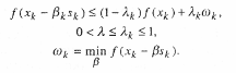
where as a value any number is chosen that satisfies the inequality
where number is any such number when ![]()
In most descent methods, the value of k is chosen to be equal to one. Thus, to determine k, one has to solve the one-dimensional minimization problem.
Gradient descent method. Since the antigradient - indicates the direction of the steepest decrease of the function f(x), then it is natural to move from the point NS k in this direction. The descent method, which is called the gradient descent method. If, then the relaxation process is called the steepest descent method.
The method of conjugate directions. In linear algebra, this method is known as the conjugate gradient method for solving systems of linear algebraic equations AX =b, and therefore, as a method of minimizing the quadratic function
Method diagram:

If = 0, then this scheme turns into a steepest descent scheme. Appropriate choice of value t k guarantees the convergence of the conjugate direction method at a rate of the same order of magnitude as in gradient descent methods and ensures that the number of iterations in quadratic descent is finite (for example).
Coordinate descent. At each iteration, as the direction of descent - s k a direction along one of the coordinate axes is selected. The method has a convergence rate of the minimization process of the order of 0 (1 / m). Moreover, it essentially depends on the dimension of the space.
Method diagram:
![]()
where the coordinate vector

If at the point x k there is information about the behavior of the gradient of the function f(x), for example:
![]()
then as the direction of descent s k we can take the coordinate vector e j . In this case, the rate of convergence of the method is n times less than with gradient descent.
At the initial stage of the minimization process, the method of cyclic coordinatewise descent can be used, when first the descent is carried out in the direction e 1 , then on e 2, etc. up to e NS , after which the whole cycle is repeated again. More promising in comparison with the previous one is the coordinate descent, in which the descent directions are chosen randomly. With this approach to the choice of direction, there are a priori estimates that guarantee for the function f(x) with the probability tending to unity at, the convergence of the process with a rate of the order of 0 (1 / m).
Method diagram:
At each step of the process, out of n numbers (1, 2, ..., n), a number is randomly selected j(k) and as s k, the unit coordinate vector e j ( k ) , after which the descent is carried out:

Random descent method.s k subject to a uniform distribution on this sphere, and then according to the element calculated at the kth step of the process NS To is determined by:

The convergence rate of the random descent method is n times lower than that of the gradient descent method, but n times higher than that of the random coordinate descent method. The considered descent methods are applicable to optional convex functions and guarantee their convergence under very small constraints on them (such as the absence of local minima).
Relaxation methods of mathematical programming. Let's return to problem 36 ((8.17) - (8.18)):
![]()
under conditions
![]()
In optimization problems with constraints, the choice of the direction of descent is associated with the need to constantly check that the new value NS k +1 should as well as the previous x k satisfy a system of constraints X.
Conditional gradient method. In this method, the idea of choosing the direction of descent is as follows: at the point NS To linearize the function f(x), constructing a linear function and then, minimizing f(x) on the set NS, find a point y k . After that, it is assumed, and further along this direction, the descent is carried out, so that
Thus, to find the direction - s k, one should solve the problem of minimizing a linear function on the set X. If X in turn is given by linear constraints, then it becomes a linear programming problem.
Possible directions method. The idea of the method: among all possible directions at a point NS To choose the one along which the function f(x) decreases the fastest, and then descend along this direction.
Direction - s at the point NS X is called possible if there is such a number that for all. To find a possible direction, it is necessary to solve a linear programming problem, or the simplest quadratic programming problem:
Under conditions:

Let be the solution to this problem. Condition (8.25) guarantees that the direction is possible. Condition (8.26) ensures the maximum value of (, that is, among all possible directions - s, direction - provides the fastest decay of the function f(x). Condition (8.27) eliminates the unboundedness of the solution to the problem. The method of possible directions is resistant to possible computational errors. However, it is difficult to estimate the rate of its convergence in the general case, and this problem still remains unsolved.
Random search method. In the general case, the implementation of the above minimization methods is very laborious, except for the simplest cases when the set of constraints has a simple geometric structure (for example, it is a multidimensional parallelepiped). In the general case, the random search method, when the direction of descent is chosen at random, can be very promising. In this case, we will significantly lose in the convergence rate, however, the simplicity of choosing the direction can compensate for these losses in terms of the total labor costs for solving the minimization problem.
Method diagram:
A random point is selected on the n-dimensional unit sphere centered at the origin r k, subject to a uniform distribution on this sphere, and then the direction of descent is s k from the conditions
Is chosen as the initial approximation. For the point calculated at each iteration x k under construction ( k+ 1) th point x k +1 :
![]()
As quality, any number from = is selected that satisfies the inequality:
The convergence of this method is proved under very loose restrictions on the function f (convexity) and many restrictions X (convexity and closedness).