Often, representatives of one species (population) feed on representatives of another species.

The Lotka - Volterra model is a model of the mutual existence of two populations of the "predator - prey" type.

The “predator-prey” model was first obtained by A. Lotka in 1925, who used it to describe the dynamics of interacting biological populations. In 1926, independently of Lotka, similar (moreover, more complex) models were developed by the Italian mathematician V. Volterra, whose deep research in the field of environmental problems laid the foundation for the mathematical theory of biological communities, or the so-called. mathematical ecology.

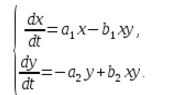
In mathematical form, the proposed system of equations has the form:

where x is the number of prey, y is the number of predators, t is time, α, β, γ, δ are coefficients that reflect interactions between populations.

Formulation of the problem

Consider an enclosed space in which there are two populations - herbivores ("prey") and carnivores. It is believed that animals are not imported or exported and that there is enough food for herbivores. Then the equation for changing the number of victims (victims only) will take the form:

where $ α $ is the birth rate of victims,

$ x $ - the size of the victim population,

$ \ frac (dx) (dt) $ - growth rate of the victim population.

When predators do not hunt, they can die out, which means that the equation for the number of predators (only predators) will take the form:

Where $ γ $ is the loss rate of predators,

$ y $ is the size of the predator population,

$ \ frac (dy) (dt) $ is the growth rate of the predator population.

When predators and prey meet (the frequency of encounters is directly proportional to the product), predators destroy prey with a coefficient, well-fed predators can reproduce offspring with a coefficient. Thus, the system of equations of the model will take the form:

The solution of the problem

Let us construct a mathematical model of the coexistence of two biological populations of the "predator-prey" type.

Let two biological populations cohabit in an isolated environment. The environment is stationary and provides an unlimited amount of everything necessary for life for one of the species - the victim. Another species - a predator - also lives in stationary conditions, but feeds only on prey. Cats, wolves, pikes, foxes can act as predators, and chickens, hares, crucians, mice, respectively, can act as victims.

For definiteness, let us consider cats in the role of predators, and chickens in the role of prey.

So, chickens and cats live in some isolated space - a farm yard. Wednesday provides unlimited food for chickens, and cats only eat chickens. Let us denote by

$ x $ - number of chickens,

$ y $ - the number of cats.

Over time, the number of chickens and cats changes, but we will consider $ x $ and $ y $ as continuous functions of time t. Let's call a pair of numbers $ x, y) $ the state of the model.

Let us find how the state of the model $ (x, y) changes. $

Consider $ \ frac (dx) (dt) $ - the rate of change in the number of chickens.

If there are no cats, then the number of chickens increases and the faster, the more chickens. We will consider the dependence to be linear:

$ \ frac (dx) (dt) a_1 x $,

$ a_1 $ is a coefficient that depends only on the living conditions of chickens, their natural mortality and fertility.

$ \ frac (dy) (dt) $ - rate of change in the number of cats (if there are no chickens), depends on the number of cats y.

If there are no chickens, then the number of cats decreases (they have no food) and they die out. We will consider the dependence to be linear:

$ \ frac (dy) (dt) - a_2 y $.

In an ecosystem, the rate of change in the number of each species will also be considered proportional to its number, but only with a coefficient that depends on the number of individuals of another species. So, for chickens, this coefficient decreases with an increase in the number of cats, and for cats, it increases with an increase in the number of chickens. We will also consider the dependence to be linear. Then we get a system of differential equations:

This system of equations is called the Volterra-Lotka model.

a1, a2, b1, b2 - numerical coefficients, which are called model parameters.

As you can see, the nature of the change in the state of the model (x, y) is determined by the values ​​of the parameters. By changing these parameters and solving the system of equations of the model, it is possible to study the patterns of changes in the state of the ecological system.

Using the MATLAB program, the Lotka-Volterra system of equations is solved as follows:

In fig. 1 shows the solution of the system. Depending on the initial conditions, the solutions are different, which corresponds to different colors of the trajectories.

In fig. 2 shows the same solutions, but taking into account the time axis t (i.e., a time dependence is observed).

PREDATOR-VICTIM COMPUTER MODEL

Kazachkov Igor Alekseevich 1, Guseva Elena Nikolaevna 2
1 Magnitogorsk State Technical University named after G.I. Nosova, Institute of Construction, Architecture and Art, 5th year student
2 Magnitogorsk State Technical University named after G.I. Nosova, Institute of Energy and Automated Systems, Candidate of Pedagogical Sciences, Associate Professor of the Department of Business Informatics and Information Technologies

COMPUTER MODEL "PREDATOR-VICTIM"

Kazatchkov Igor Alekseevich 1, Guseva Elena Nikolaevna 2
1 Nosov Magnitogorsk State Technical University, Civil Engineering, Architecture and Arts Institute, student of the 5th course
2 Nosov Magnitogorsk State Technical University, Power Engineering and Automated Systems Institute, PhD in Pedagogical Science, Associate Professor of the Business Computer Science and Information Technologies Department

Environmental modeling is used to study our environment. Mathematical models are used in cases where there is no natural environment and no natural objects, it helps to predict the influence of various factors on the object under study. This method takes over the functions of checking, constructing and interpreting the results obtained. On the basis of such forms, ecological modeling is concerned with the assessment of changes in our environment.

At the moment, such forms are used to study the environment around us, and when it is required to study any of its areas, then mathematical modeling is used. This model makes it possible to predict the influence of certain factors on the object of study. At one time, the type "predator - prey" was proposed by such scientists as: T. Malthus (Malthus 1798, Malthus 1905), Verhulst (Verhulst 1838), Pearl (Pearl 1927, 1930), as well as A. Lotka (Lotka 1925, 1927 ) and V. Volterra (Volterra 1926). These models reproduce the periodic oscillatory regime arising as a result of interspecies interactions in nature.

One of the main methods of cognition is modeling. In addition to the fact that it can predict changes in the environment, it also helps to find the best way to solve the problem. For a long time, in ecology, mathematical models have been used in order to establish patterns, trends in the development of populations, help to highlight the essence of observations. The layout can serve as a sample behavior, object.

When reconstructing objects in mathematical biology, predictions of various systems are used, special individualities of biosystems are provided: the internal structure of an individual, life support conditions, the constancy of ecological systems, thanks to which the vital activity of systems is saved.
The advent of computer modeling has significantly pushed the frontier of research ability. There was a possibility of multilateral implementation of difficult forms that did not allow analytical study, new directions appeared, as well as simulation modeling.

Let's consider what a modeling object is. “The object is a closed habitat where two biological populations interact: predators and prey. The process of growth, extinction and reproduction takes place directly on the surface of the habitat. The food of the prey occurs at the expense of the resources that are present in the given environment, and the food of the predators is at the expense of the prey. At the same time, nutritional resources can be both renewable and non-renewable.

In 1931, Vito Volterra deduced the following laws of the predator-prey relationship.

The law of the periodic cycle - the process of destruction of prey by a predator often leads to periodic fluctuations in the population size of both species, depending only on the growth rate of carnivores and herbivores, and on the initial ratio of their numbers.

The law of conservation of mean values ​​is that the average number of each species is constant, regardless of the initial level, provided that the specific rates of increase in the number of populations, as well as the efficiency of predation, are constant.

The law of violation of the average values ​​- with a decrease in both species in proportion to their number, the average population of the prey grows, and the number of predators decreases.

The predator-prey model is a special relationship of predator with prey, as a result of which both win. The healthiest and most adapted individuals survive, i.e. all this is due to natural selection. In an environment where there is no opportunity for reproduction, the predator will sooner or later destroy the prey population, after which it will die out itself. "

There are many living organisms on earth, which, under favorable conditions, increase the number of congeners to an enormous scale. This ability is called: the biotic potential of the species, i.e. an increase in the number of species over a certain period of time. Each species has its own biotic potential, for example, large species of organisms can grow only 1.1 times per year, while organisms of smaller species, such as crustaceans, etc. can enlarge their appearance up to 1030 times, and bacteria in even greater numbers. In any of these cases, the population will grow exponentially.

The exponential growth of the population is called the geometric progression of the growth of the population. This ability can be observed in the laboratory in bacteria, yeast. In non-laboratory conditions, exponential growth can be seen in the example of locusts or other species of insects. Such an increase in the number of the species can be observed in those places where it has practically no enemies, and there is more than enough food. Eventually, the increase in the species, after the numbers increased for a short time, the growth of the population began to decline.

Consider a computer model of mammalian reproduction using the Lotka-Volterra model as an example. Let in some territory there are two types of animals: deer and wolves. Mathematical model of changes in population size in the model Volterra Trays:

The initial number of victims is xn, the number of predators is yn.

Model parameters:

P1 - the probability of meeting a predator,

P2 is the growth rate of predators at the expense of prey,

d is the mortality rate of predators,

a is the growth rate of the number of victims.

In the educational task, the following values ​​were set: the number of deer was 500, the number of wolves was 10, the growth rate of deer was 0.02, the growth rate of the number of wolves was 0.1, the probability of meeting a predator was 0.0026, and the growth rate of predators due to prey was 0 , 000056. The data is calculated for 203 years.

Exploring the impact the growth rate of victims for the development of two populations, the remaining parameters will be left unchanged. Scheme 1 shows an increase in the number of prey and then, with some delay, an increase in predators is observed. Then the predators knock out the prey, the number of prey drops sharply, followed by a decrease in the number of predators (Fig. 1).

Figure 1. Population size with low fertility among victims

Let us analyze the change in the model by increasing the victim's fertility rate a = 0.06. In Scheme 2, we see a cyclical oscillatory process leading to an increase in the size of both populations over time (Fig. 2).

Figure 2: Population size with mean fertility rate among victims

Let us consider how the dynamics of populations will change with a high value of the fertility rate of the victim a = 1.13. In fig. 3, a sharp increase in the number of both populations is observed, followed by the extinction of both prey and predator. This is due to the fact that the number of the victim population has increased to such an amount that resources have begun to run out, as a result of which the prey becomes extinct. The extinction of predators occurs due to the fact that the number of victims has decreased and the predators have run out of resources for their existence.

Figure 3 Population size with high fertility in victims

Based on the analysis of the data of a computer experiment, it can be concluded that computer modeling allows us to predict the size of populations, to study the influence of various factors on population dynamics. In the given example, we investigated the “predator-prey” model, the influence of the prey birth rate on the number of deer and wolves. A small increase in the prey population leads to a slight increase in prey, which after a certain period is destroyed by predators. A moderate increase in the prey population leads to an increase in the size of both populations. A high increase in the prey population first leads to a rapid increase in the prey population, this affects the increase in the growth of predators, but then the prolific predators quickly destroy the deer population. As a result, both species become extinct.

Back in the 20s. A. Lotka, and a little later independently of him V. Volterra proposed mathematical models describing the conjugate fluctuations in the numbers of predator and prey populations. Let's consider the simplest version of the Lotka-Volterra model. The model is based on a number of assumptions:

1) the prey population grows exponentially in the absence of a predator,

2) the press of predators inhibits this growth,

3) the mortality of the prey is proportional to the frequency of encounters between the predator and the prey (or otherwise, proportional to the product of the densities of their populations);

4) the birth rate of a predator depends on the intensity of consumption of prey.

The instantaneous rate of change in the size of the prey population can be expressed by the equation

dN w / dt = r 1 N w - p 1 N w N x,

where r 1 - specific instantaneous rate of prey population growth, p 1 is a constant linking prey mortality with the predator density, a N w and N x - density of prey and predator, respectively.

The instantaneous growth rate of the predator population in this model is taken to be equal to the difference between fertility and constant mortality:

dN x / dt = p 2 N w N x - d 2 N x,

where p 2 - constant linking the fertility in the predator population with the density of prey, a d 2 - specific mortality of a predator.

According to the above equations, each of the interacting populations in its increase is limited only by the other population, i.e. an increase in the number of prey is limited by the pressure of predators, and an increase in the number of predators is limited by an insufficient number of prey. No self-limitation of populations is expected. It is believed, for example, that there is always enough food for the victim. It is also not expected that the prey population will get out of the control of the predator, although in fact this happens quite often.

Despite all the conventionality of the Lotka-Volterra model, it deserves attention if only because it shows how even such an idealized system of interaction between two populations can generate a rather complex dynamics of their numbers. The solution of the system of these equations makes it possible to formulate the conditions for maintaining a constant (equilibrium) number of each of the species. The prey population remains constant if the density of the predator is equal to r 1 / p 1, and in order for the population of the predator to remain constant, the prey density must be equal to d 2 / p 2. If we plot the density of victims on the abscissa axis N f , and the ordinate is the density of the predator N X, then the isoclines showing the condition of the constancy of the predator and prey will be two straight lines perpendicular to each other and coordinate axes (Fig. 6, a). It is assumed that below a certain (equal to d 2 / p 2) density of prey, the density of the predator will always decrease, and above it, it will always increase. Accordingly, the density of the prey increases if the density of the predator is lower than the value equal to r 1 / p 1, and decreases if it is higher than this value. The point of intersection of the isoclines corresponds to the condition of the constancy of the numbers of predators and prey, while other points on the plane of this graph move along closed trajectories, thus reflecting regular fluctuations in the numbers of predators and prey (Fig. 6, b). The range of fluctuations is determined by the initial ratio of the densities of the predator and prey. The closer it is to the point of intersection of the isoclines, the smaller the circle described by the vectors, and, accordingly, the smaller the vibration amplitude.

Rice. 6. Graphic expression of the Lotka-Voltaire model for the predator-prey system.

One of the first attempts to obtain fluctuations in the number of predators and prey in laboratory experiments was made by G.F. Gause. The objects of these experiments were the ciliate Paramecia (Paramecium caudatum) and predatory ciliate didinium (Didinium nasutum). A suspension of bacteria regularly introduced into the medium served as food for the Paramecia, and didinium ate only Paramecia. This system turned out to be extremely unstable: the pressure of the predator, as its number increased, led to the complete extermination of the prey, after which the population of the predator itself died out. Complicating the experiments, Gause arranged a refuge for the victim, adding a little glass wool to the test tubes with ciliates. Paramecia could move freely among the cotton wool, but didiniums could not. In this version of the experiment, the didinium ate all the Paramecia floating in the cotton-free part of the test tube and died out, and the Paramecia population then recovered due to the reproduction of individuals that survived in the shelter. Some similarity of fluctuations in the number of predators and prey was achieved by Gauze only when he introduced both prey and predator into the culture from time to time, thus imitating immigration.

40 years after Gause's work, his experiments were repeated by L. Luckinbill, who used ciliates as a victim. Paramecium aurelia, but as a predator of the same Didinium nasutum. Luckinbill managed to obtain several cycles of fluctuations in the number of these populations, but only in the case when the density of Paramecia was limited by a lack of food (bacteria), and methylcellulose was added to the culture liquid - a substance that reduces the speed of movement of both the predator and the prey and therefore reduces the frequency of their possible meetings. It also turned out that it is easier to achieve oscillations between the predator and the prey if the volume of the experimental vessel is increased, although the condition for food limitation of the prey is also mandatory in this case. If, however, excess food was added to the system of predator and prey coexisting in an oscillatory mode, then the answer was a rapid increase in the number of prey, followed by an increase in the number of the predator, leading in turn to the complete extermination of the prey population.

The Lotka and Volterra models served as the impetus for the development of a number of other more realistic models of the predator-prey system. In particular, a fairly simple graphical model that analyzes the ratio of different isoclines of the victim predator, was proposed by M. Rosenzweig and R. MacArthur (Rosenzweig, MacArthur). According to these authors, stationary ( = constant) the number of prey in the coordinate axes of the density of the predator and prey can be represented as a convex isocline (Fig. 7, a). One point of intersection of the isocline with the prey density corresponds to the minimum allowable prey density (the lower population is at a very high risk of extinction, if only because of the low frequency of meetings of males and females), and the other, the maximum, determined by the amount of food available or the behavioral characteristics of the prey itself. We emphasize that we are talking so far about the minimum and maximum densities in the absence of a predator. With the appearance of a predator and an increase in its number, the minimum permissible prey density, obviously, should be higher, and the maximum - lower. Each value of the prey density must correspond to a certain density of the predator, at which the constancy of the prey population is achieved. The locus of such points is the isocline of the prey in the coordinates of the density of the predator and prey. The vectors showing the direction of the change in the density of the victim (oriented horizontally) have different directions on different sides of the isocline (Fig. 7, a).

Rice. 7. Isoclines of stationary populations of prey (a) and predator (b).

An isocline corresponding to the stationary state of its population was also plotted for the predator in the same coordinates. The vectors showing the direction of the change in the number of the predator are oriented up or down, depending on which side of the isocline they are on. The shape of the predator isocline shown in Fig. 7, b. is determined, firstly, by the presence of a certain minimum density of the prey, sufficient to maintain the population of the predator (at a lower density of the prey, the predator cannot increase its number), and secondly, by the presence of a certain maximum density of the predator itself, above which the number will decrease independently from the abundance of victims.

Rice. 8. The emergence of oscillatory regimes in the predator-prey system depending on the location of the isoclines of the predator and prey.

When combining prey and predator isoclines on the same graph, three different options are possible (Fig. 8). If the isocline of a predator crosses the isocline of the prey in the place where it is already decreasing (at a high density of prey), the vectors showing the change in the numbers of the predator and prey form a trajectory twisting inward, which corresponds to the decaying fluctuations in the number of prey and predator (Fig. 8, a). In the case when the isocline of the predator crosses the isocline of the prey in its ascending part (i.e., in the region of low values ​​of the density of prey), the vectors form an unwinding trajectory, and the fluctuations in the numbers of the predator and prey occur, respectively, with an increasing amplitude (Fig. 8, b). If the isocline of a predator crosses the isocline of the prey in the region of its apex, then the vectors form a closed circle, and the fluctuations in the numbers of prey and predator are characterized by a stable amplitude and period (Fig. 8, v).

In other words, damped oscillations correspond to a situation in which a predator has a tangible effect on the prey population, which has reached only a very high density (close to the limiting one), and oscillations of increasing amplitude arise when the predator is able to rapidly increase its number even with a low prey density, and so destroy it quickly. In other versions of their model, Posenzweig and MacArthur showed that it is possible to stabilize the oscillations of a predator-prey by introducing a “refuge”, i.e. assuming that in an area of ​​low prey density, there is an area where prey numbers grow regardless of the number of predators available.

The desire to make models more realistic by complicating them manifested itself in the works of not only theorists, but also experimenters. In particular, interesting results were obtained by Huffaker, who showed the possibility of coexistence of a predator and prey in an oscillatory mode using the example of a small herbivorous tick Eotetranychus sexmaculatus and a predatory mite attacking it Typhlodromus occidentalis. Oranges were used as food for the herbivorous mite, placed on trays with holes (such as those used for storing and transporting eggs). Originally, there were 40 holes on one tray, some containing oranges (partially peeled) and others containing rubber balls. Both types of ticks reproduce parthenogenetically very quickly, and therefore the nature of their population dynamics can be identified in a relatively short time. Having placed 20 females of herbivorous ticks on a tray, Haffaker observed a rapid increase in its population, which stabilized at the level of 5-8 thousand individuals (per orange). If several individuals of the predator were added to the growing population of the prey, then the population of the latter rapidly increased in number and died out when all the prey were eaten.

By increasing the size of the tray to 120 holes, in which individual oranges were randomly scattered among many rubber balls, Huffaker was able to prolong the coexistence of predator and prey. An important role in the interaction of predator and prey, as it turned out, is played by the ratio of the rates of their dispersal. Huffaker suggested that by making it easier for the prey to move and making it harder for the predator to move, it would be possible to increase the time of their coexistence. To do this, 6 oranges were randomly placed on a tray of 120 holes among rubber balls, and around the holes with oranges were arranged vaseline barriers that prevented the predator from settling, and to facilitate the settling of the victim, wooden pegs were attached to the tray, which served as a kind of "take-off pads" for herbivorous mites (the fact is that this species produces thin threads and with their help it can float in the air, spreading in the wind). In such a complicated habitat, the predator and prey coexisted for 8 months, demonstrating three complete cycles of abundance fluctuations. The most important conditions for this coexistence are as follows: heterogeneity of the habitat (in the sense of the presence in it of areas suitable and unsuitable for prey habitation), as well as the possibility of migration of prey and predator (with preservation of some prey advantage in the speed of this process). In other words, a predator can completely exterminate one or another local accumulation of prey, but some of the individuals of the prey will have time to migrate and give rise to other local accumulations. Sooner or later, the predator will also reach new local clusters, but in the meantime the prey will have time to settle in other places (including those where it lived before, but was then exterminated).

Something similar to what Huffaker observed in the experiment is also found in natural conditions. So, for example, the cactus moth butterfly (Cactoblastis cactorum), brought to Australia, significantly reduced the number of prickly pear cactus, but did not completely destroy it precisely because the cactus manages to settle a little faster. In those places where the prickly pear is completely exterminated, the moth ceases to occur. Therefore, when after a while the prickly pear again penetrates here, then within a certain period it can grow without the risk of being destroyed by the moth. Over time, however, the moth reappears here and, multiplying rapidly, destroys the prickly pear.

Speaking about the predator-prey fluctuations, one cannot fail to mention the cyclical changes in the number of hares and lynxes in Canada, traced from the statistics of fur procurement by the Hudson Bay Company from the end of the 18th to the beginning of the 20th century. This example has often been viewed as a classic illustration of predator-prey fluctuations, although in reality we only see the growth of the predator (lynx) population following the growth of the prey (hare). As for the decrease in the number of hares after each rise, it could not be explained only by the increased pressure of predators, but was associated with other factors, apparently, first of all, the lack of food in winter. This conclusion was reached, in particular, by M. Gilpin, who tried to check whether these data can be described by the classical Lotka-Volterra model. The test results showed that there was no satisfactory fit to the model, but oddly enough, it became better if the predator and prey were interchanged, i.e. the lynx was treated as a "prey" and the hare as a "predator". A similar situation was reflected in the joking title of the article ("Do hares eat lynxes?"), Which was essentially very serious and published in a serious scientific journal.

Predator-Prey Situation Model

Let us consider a mathematical model of the dynamics of the coexistence of two biological species (populations) interacting with each other according to the "predator-prey" type (wolves and rabbits, pikes and crucians, etc.), called the Volter-Lotka model. It was first obtained by A. Lotka (1925), and a little later and independently of Lotka, similar and more complex models were developed by the Italian mathematician V. Volterra (1926), whose work actually laid the foundations of the so-called mathematical ecology.

Let there be two biological species that live together in an isolated environment. This assumes:

• 1. The victim can find enough food to feed;
• 2. At each meeting of the prey with the predator, the latter kills the prey.

For the sake of definiteness, we will call them crucians and pikes. Let

the state of the system is determined by the quantities x (t) and y (t)- the number of crucians and pikes at a time G. To obtain mathematical equations that approximately describe the dynamics (change over time) of the population, we will proceed as follows.

As in the previous model of population growth (see Section 1.1), for victims we have the equation

where a> 0 (fertility exceeds mortality)

Coefficient a the growth of prey depends on the number of predators (decreases with their increase). In the simplest case a - a - fjy (a> 0, p> 0). Then for the size of the victim population we have the differential equation

For the population of predators, we have the equation

where b> 0 (death rate exceeds birth rate).

Coefficient b the decline of predators decreases if there are prey to eat. In the simplest case, you can take b - y -Sx (y > 0, S> 0). Then for the size of the population of predators we obtain the differential equation

Thus, equations (1.5) and (1.6) represent a mathematical model of the considered problem of interaction between populations. In this model, the variables x, y- the state of the system, and the coefficients characterize its structure. The nonlinear system (1.5), (1.6) is the Voltaire-Lotka model.

Equations (1.5) and (1.6) should be supplemented with initial conditions - given values ​​of initial populations.

Let us now analyze the constructed mathematical model.

Let us construct the phase portrait of system (1.5), (1.6) (in the sense of the problem X> 0, v> 0). Dividing equation (1.5) by equation (1.6), we obtain an equation with separable variables

By ignoring this equation, we have

Relation (1.7) gives the equation of phase trajectories in an implicit form. System (1.5), (1.6) has a stationary state determined from

From equations (1.8) we obtain (since l * F 0, y * F 0)

Equalities (1.9) determine the equilibrium position (point O)(Fig. 1.6).

The direction of motion along the phase trajectory can be determined from such considerations. Let the carp be few. G. e. x ~ 0, then from equation (1.6) y

All phase trajectories (except for the point 0) closed curves covering the equilibrium position. The state of equilibrium corresponds to a constant number x "and y" of crucian carp and pike. Crucian carps breed, pike eat them, die out, but the number of those and others does not change. "Closed phase trajectories correspond to a periodic change in the number of crucians and pikes. Moreover, the trajectory along which the phase point moves depends on the initial conditions. Consider how the state changes along the phase trajectory. Let the point be in the position A(fig. 1.6). There are few crucians, a lot of pikes; pikes have nothing to eat, and they are gradually dying out and almost

disappear completely. But the number of crucians also decreases to almost zero and

only later, when the pike became less than at, the increase in the number of crucians begins; the rate of their growth increases and their number increases - this happens to about a point V. But an increase in the number of crucians leads to inhibition of the extinction process of shuk and their number begins to grow (there is more food) - the site Sun. Then there are a lot of pikes, they eat crucian carp and eat almost all of them (site CD). After that, the pikes begin to die out again and the process repeats with a period of about 5-7 years. In fig. 1.7 qualitatively plotted curves of changes in the number of crucians and pikes, depending on time. The maxima of the curves alternate, with the maxima of the abundance of pikes lagging behind the maxima of crucian carp.

This behavior is typical for various systems of the predator-prey type. Let us now interpret the results obtained.

Despite the fact that the considered model is the simplest and in reality everything is much more complicated, it made it possible to explain some of the mysterious that exists in nature. The stories of fishermen about the periods when "the pikes themselves jump into their hands" are understandable;

Note one more interesting conclusion that can be drawn from Fig. 1.6. If at the point R there is a quick catch of pikes (in another terminology - shooting wolves), then the system "jumps" to the point Q, and further movement occurs along a closed trajectory of a smaller size, which is intuitively expected. If we decrease the number of pikes at the point R, then the system will go to point S, and further movement will follow a larger trajectory. The vibration amplitudes will increase. This is contrary to intuition, but it just explains this phenomenon: as a result of shooting wolves, their number increases over time. Thus, the choice of the moment of shooting is important in this case.

Suppose two populations of insects (for example, the aphid and the ladybug, which is aphid) were in natural equilibrium x-x *, y = y *(dot O in Fig. 1.6). Consider the impact of a single application of an insecticide that kills x> 0 of the victims and y> 0 of the predators without destroying them completely. A decrease in the number of both populations leads to the fact that the representative point from the position O Will "jump" closer to the origin, where x> 0, y 0 (Fig. 1.6) It follows that as a result of the action of the insecticide designed to destroy the victims (aphids), the number of victims (aphids) increases, and the number of predators (ladybirds) decreases. It turns out that the number of predators can become so small that they will be fond of complete extinction, but for other reasons (drought, disease, etc.). Thus, the use of insecticides (unless they almost completely destroy harmful insects) ultimately leads to an increase in the population of those insects whose numbers were under the control of other predatory insects. Such cases are described in books on biology.

In the general case, the growth rate of the number of victims a depends on both L "and y: a= a (x, y) (due to the presence of predators and due to food restrictions).

With a small change in model (1.5), (1.6), small terms are added to the right-hand sides of the equations (taking into account, for example, the competition of carp for food and pike for carp)

here 0 f.i «1.

In this case, the conclusion about the periodicity of the process (the return of the system to its original state), which is valid for the model (1.5), (1.6), loses its validity. Depending on the type of small corrections / and g the situations shown in Fig. 1.8.

In case (1), the equilibrium state O stable. For any other initial conditions, it is precisely this that is established after a sufficiently long time.

In case (2), the system is "running out of gear". The stationary state is unstable. Such a system eventually falls into such a range of values X and y, that the model is no longer applicable.

In case (3) in a system with an unstable stationary state O a periodic mode is established over time. In contrast to the original model (1.5), (1.6), in this model, the steady-state periodic regime does not depend on the initial conditions. Initially small deviation from steady state O leads not to small fluctuations about O, as in the Volterra-Lotka model, but to oscillate a completely definite (and not depending on the small deviation) amplitude.

IN AND. Arnold calls the Volterra-Lotka model rigid, because its small change can lead to conclusions different from those given above. To judge which of the situations indicated in Fig. 1.8, is implemented in this system, additional information about the system is absolutely necessary (about the form of small corrections / and g).

In the Kolmogorov model, one significant assumption is made: since it is assumed that this means the existence of mechanisms in the prey population that regulate their numbers even in the absence of predators.

Unfortunately, such a formulation of the model does not allow answering the question around which there has been a lot of controversy and which we already mentioned at the beginning of the chapter: how can a population of predators have a regulatory effect on the population of prey so that the entire system is stable? Therefore, we return to model (2.1), in which there are no self-regulation mechanisms (for example, regulation by means of intraspecific competition) in the prey population (as well as in the predator population); therefore, the only mechanism for the regulation of the numbers included in the species community is the trophic relationship between predators and prey.

Here (so that, unlike the previous model, Naturally, solutions (2.1) depend on the specific type of trophic function, which, in turn, is determined by the nature of predation, i.e., the trophic strategy of the predator and the protective strategy of the prey. functions (see Fig. I) are the following properties:

System (2.1) has one nontrivial stationary point, the coordinates of which are determined from the equations

under natural limitation.

There is one more stationary point (0, 0) corresponding to a trivial equilibrium. It is easy to show that this point is a saddle, and the coordinate axes are the separatrices.

The characteristic equation for a point has the form

Obviously, for the classical Volterra model.

Therefore, the value of f can be regarded as a measure of the deviation of the considered model from the Volterra one.

a stationary point is a focus, and oscillations appear in the system; when the opposite inequality is fulfilled, there is a knot, and there are no oscillations in the system. The stability of this equilibrium state is determined by the condition

that is, it essentially depends on the type of trophic function of the predator.

Condition (5.5) can be interpreted as follows: for the stability of the nontrivial equilibrium of the predator - prey system (and thus, for the existence of this system), it is sufficient that in the vicinity of this state the relative proportion of prey consumed by the predator increases with the number of prey. Indeed, the proportion of prey (of their total number) consumed by a predator is described by a differentiable function whose growth condition (positive derivative) looks like

The last condition taken at the point is nothing but condition (5.5) for equilibrium stability. If it is continuous, it should also be fulfilled in some neighborhood of the point.Thus, if the number of victims in this neighborhood, then

Now let the trophic function V have the form shown in Fig. 11, a (typical for invertebrates). It can be shown that for all finite values ​​(since it is convex upward)

that is, for any values ​​of the stationary number of victims, inequality (5.5) does not hold.

This means that in a system with this type of trophic function, there is no stable non-trivial equilibrium. Several outcomes are possible: either the numbers of both the prey and the predator increase indefinitely, or (when passing the trajectory near one of the coordinate axes), due to random reasons, the number of prey or the number of the predator will become equal to zero. If the prey dies, the predator will also die after a while, but if the predator dies first, the number of the prey will begin to grow exponentially. The third option - the emergence of a stable limit cycle - is impossible, which is easily proved.

Indeed, the expression

in the positive quadrant is always positive, if only has the form shown in Fig. 11, a. Then, according to the Dulac criterion, there are no closed trajectories in this area and a stable limit cycle cannot exist.

So, we can conclude: if the trophic function has the form shown in Fig. 11, a, then the predator cannot be a regulator that ensures the stability of the prey population and thus the stability of the entire system as a whole. The system can be stable only if the victim population has its own internal regulatory mechanisms, for example, intraspecific competition or epizootics. This regulation option has already been considered in §§ 3, 4.

Earlier it was noted that this type of trophic function is characteristic of insect predators, whose "victims" are also usually insects. On the other hand, observations of the dynamics of many natural communities of the "predator-prey" type, which include insect species, show that they are characterized by fluctuations of a very large amplitude and of a very specific type.

Usually, after a more or less gradual increase in the number (which can occur either monotonously or in the form of fluctuations with an increasing amplitude), its sharp drop occurs (Fig. 14), and then the pattern repeats. Apparently, this nature of the dynamics of the number of insect species can be explained by the instability of this system at low and medium values ​​of the number and the action of powerful intrapopulation regulators of the number at its large values.

Rice. 14. Population dynamics of the Australian leaf beetle Cardiaspina albitextura feeding on eucalyptus trees. (From: Clark L. R. The population dynamics of Cardiaspina albitextura.-Austr. J. Zool., 1964, 12, no. 3, p. 362-380.)

If the "predator - prey" system includes species capable of rather complex behavior (for example, predators are capable of learning or prey are capable of finding refuge), then in such a system a stable non-trivial equilibrium may exist. The proof of this statement is quite simple.

Indeed, the trophic function should then have the form shown in Fig. 11, c. The point on this graph is the point of tangency of the straight line drawn from the origin to the graph of the trophic function. Obviously, at this point the function has a maximum. It is also easy to show that condition (5.5) is satisfied for all. Consequently, a nontrivial equilibrium in which the number of victims is less will be asymptotically stable

However, we cannot say anything about how large the region of stability of this equilibrium is. For example, if there is an unstable limit cycle, then this area must lie within the cycle. Or another option: nontrivial equilibrium (5.2) is unstable, but there is a stable limit cycle; in this case, we can also talk about the stability of the predator-prey system. Since expression (5.7), when choosing a trophic function of the type in Fig. 11, в can change sign when changing at, then the Dulac criterion does not work here and the question of the existence of limit cycles remains open.