
Characteristic equation of a system of differential equations. Systems of differential equations. This system can be represented as
Many systems differential equations, both homogeneous and inhomogeneous, can be reduced to a single equation for a single unknown function. Let's show the method with examples.
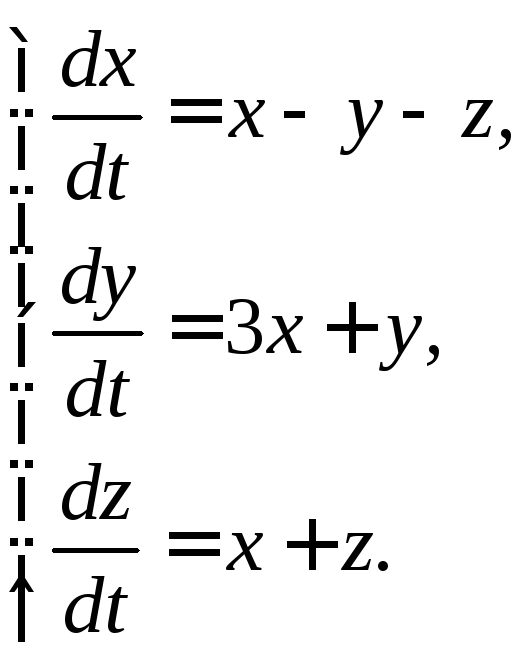
Example 3.1. Solve the system
Solution. 1) Differentiating with respect to t first equation and using the second and third equations to replace And  , we find
The resulting equation is differentiable with respect to  again
again
1) We make a system

From the first two equations of the system, we express the variables  And
And  through
  :
:
Let us substitute the found expressions for  And
And  into the third equation of the system
So, to find the function  obtained a third-order differential equation with constant coefficients
 .
.
2) We integrate the last equation by the standard method: we compose the characteristic equation  , find its roots
  and build a general solution in the form of a linear combination of exponentials, taking into account the multiplicity of one of the roots:.
3) Next to find the two remaining features  And
And  , we differentiate the twice obtained function
Using connections (3.1) between the system functions, we recover the remaining unknowns
 .
.
Answer.
, ,.
,.
It may turn out that all known functions except one are excluded from the third-order system even after a single differentiation. In this case, the order of the differential equation for finding it will be less than the number of unknown functions in the original system.
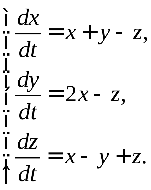
Example 3.2. Integrate the system
 (3.2)
(3.2)
Solution. 1) Differentiating with respect to  first equation, we find
Excluding variables  And
And  from the equations

we will have a second-order equation with respect to 
 (3.3)
(3.3)
2) From the first equation of system (3.2) we have
 (3.4)
(3.4)
Substituting into the third equation of system (3.2) the found expressions (3.3) and (3.4) for  And
And  , we obtain a first-order differential equation to determine the function

Integrating this inhomogeneous equation with constant first-order coefficients, we find  Using (3.4), we find the function
Answer.
 ,,
,, .
.
Task 3.1. Solve homogeneous systems by reducing to one differential equation.
3.1.1. 3.1.2.
3.1.3.
 3.1.4.

3.1.5.
 3.1.6.

3.1.7.
 3.1.8.

3.1.9.
 3.1.10.

3.1.11.
 3.1.12.

3.1.13.
 3.1.14.
3.1.15.
 3.1.16.

3.1.17.
 3.1.18.

3.1.19.
 3.1.20.

3.1.21.
 3.1.22.

3.1.23.
 3.1.24.

3.1.25.
 3.1.26.

3.1.27.
 3.1.28.

3.1.29.
 3.1.30.

3.2. Solving systems of linear homogeneous differential equations with constant coefficients by finding a fundamental system of solutions
The general solution of a system of linear homogeneous differential equations can be found as a linear combination of the fundamental solutions of the system. In the case of systems with constant coefficients, linear algebra methods can be used to find fundamental solutions.
Example 3.3. Solve the system
 (3.5)
(3.5)
Solution. 1) Rewrite the system in matrix form
 . (3.6)
2) We will look for a fundamental solution of the system in the form of a vector  . Substituting functions
  in (3.6) and reducing by
  , we get

 , (3.7)
that is the number  must be an eigenvalue of the matrix
  , and the vector
  corresponding eigenvector.
3) From the course of linear algebra, it is known that the system (3.7) has a non-trivial solution if its determinant is equal to zero
 ,
,
that is . From here we find the eigenvalues  .
.
4) Find the corresponding eigenvectors. Substituting into (3.7) the first value  , we obtain a system for finding the first eigenvector


From here we get the connection between the unknowns  . It is enough for us to choose one non-trivial solution. Assuming
  , Then
  , that is, the vector
  is eigenvalue for eigenvalue
  , and the function vector
  fundamental solution of the given system of differential equations (3.5). Similarly, when substituting the second root
  in (3.7) we have the matrix equation for the second eigenvector
  . Where do we get the connection between its components
  . Thus, we have the second fundamental solution
 .
.
5) The general solution of system (3.5) is constructed as a linear combination of two obtained fundamental solutions

or in coordinate form

 .
.
Answer.

 .
.
Task 3.2. Solve systems by finding the fundamental system of solutions.
Basic concepts and definitions the simplest task dynamics of a point: the forces acting on a material point are given; find the law of motion, i.e., find the functions x = x(t), y = y(t), z = z(t), expressing the dependence of the coordinates of the moving point on time. The system resulting from this general case has the form Here x, y, z are the coordinates of the moving point, t is the time, f,g,h are known functions of their arguments. A system of the form (1) is called canonical. Turning to the general case of a system of m differential equations with m unknown functions of the argument t, we call a system of the form resolved with respect to higher derivatives canonical. The system of first-order equations resolved with respect to the derivatives of the desired functions is called normal. If taken as new auxiliary functions, then the general canonical system (2) can be replaced by an equivalent normal system consisting of equations. Therefore, it suffices to consider only normal systems. For example, one equation is a special case of the canonical system. Setting ^ = y, by virtue of the original equation we will have As a result, we obtain a normal system of equations SYSTEMS OF DIFFERENTIAL EQUATIONS Integration methods Elimination methods Method of integrable combinations Systems of linear differential equations Fundamental matrix Method of variation of constants Systems of linear differential equations with constant coefficients Matrix method equivalent to the original equation. Definition 1. The solution of the normal system (3) on the interval (a, b) of the change of the argument t is any system of n functions "differentiable on the interval that converts the equations of system (3) into identities with respect to t on the interval (a, b). The Cauchy problem for of system (3) is formulated as follows: find a solution (4) of the system that satisfies the initial conditions for t = to dimensional domain D of changes in the variables t, X\, x 2, ..., xn. If there exists a neighborhood ft fine in which the functions ft are continuous in the set of arguments and have bounded partial derivatives with respect to the variables X1, x2, ..., xn, then there is an interval to - L0 of change in t on which there exists a unique solution of the normal system (3) that satisfies the initial conditions of the Cauchy problem, if 1) for any admissible values, the system of functions (6) turns equations (3) into identities, 2) in the domain П functions (6) solve any Cauchy problem. Solutions obtained from the general for specific values of the constants are called particular solutions. For clarity, let us turn to the normal system of two equations. We will consider the system of values t> X\, x2 as rectangular Cartesian coordinates points of three-dimensional space referred to the Otx\x2 coordinate system. The solution of system (7), which takes values at t - to, determines in space a certain line passing through a point) - This line is called the integral curve of the normal system (7). The Ko-shi problem for system (7) receives the following geometric formulation: in the space of variables t > X\, x2, find the integral curve passing through the given point Mo(to,x1,x2) (Fig. 1). Theorem 1 establishes the existence and uniqueness of such a curve. The normal system (7) and its solution can also be given the following interpretation: we will consider the independent variable t as a parameter, and the solution of the system as parametric equations of a curve in the x\Ox2 plane. This plane of variables X\X2 is called the phase plane. In the phase plane, the solution (0 of system (7), which at t = t0 takes initial values x°(, x2, is represented by the curve AB passing through the point). This curve is called the trajectory of the system (phase trajectory). The trajectory of system (7) is the projection of the integral curve onto the phase plane. From the integral curve, the phase trajectory is uniquely determined, but not vice versa. § 2. Methods for integrating systems of differential equations 2.1. Elimination Method One of the integration methods is the elimination method. A special case of the canonical system is one equation of the nth order, solved with respect to the highest derivative. Introducing the new functions of the equation by the following normal system of n equations: replace this one equation of the nth order is equivalent to the normal system (1). The converse can also be asserted, that, generally speaking, a normal system of n first-order equations is equivalent to one equation of order n. This is the basis of the elimination method for integrating systems of differential equations. It is done like this. Let we have a normal system of differential equations Let us differentiate the first of equations (2) with respect to t. We have Replacing on the right side of the product or, in short, Equation (3) is again differentiable with respect to t. Taking system (2) into account, we obtain or Continuing this process, we find Suppose that the determinant (the Jacobian of the system of functions is nonzero for the considered values Then the system of equations composed of the first equation of system (2) and the equations will be solvable with respect to the unknowns will be expressed through Introducing the found expressions into the equation we get one equation of the nth order. From the very method of its construction it follows that if) there are solutions to system (2), then the function X\(t) will be a solution to equation (5). Conversely, let be the solution of equation (5). Differentiating this solution with respect to t, we calculate and substitute the found values as known functions. By assumption, this system can be solved with respect to xn as a function of t. It can be shown that the system of functions constructed in this way constitutes a solution to the system of differential equations (2). Example. It is required to integrate the system Differentiating the first equation of the system, we have whence, using the second equation, we obtain - a second-order linear differential equation with constant coefficients with one unknown function. Its general solution has the form By virtue of the first equation of the system, we find the function. The found functions x(t), y(t), as it is easy to check, for any values of С| and C2 satisfy the given system. The functions can be represented in the form from which it can be seen that the integral curves of system (6) are helical lines with a step with a common axis x = y = 0, which is also an integral curve (Fig. 3). Eliminating the parameter in formulas (7), we obtain an equation so that the phase trajectories of a given system are circles centered at the origin - projections of helical lines onto a plane. At A = 0, the phase trajectory consists of one point, called the rest point of the system. ". It may turn out that the functions cannot be expressed in terms of Then the equations of the nth order, equivalent to the original system, we will not get. Here is a simple example. The system of equations cannot be replaced by an equivalent second-order equation for x\ or x2. This system is composed of a pair of 1st order equations, each of which is independently integrated, which gives the Method of integrable combinations Integration of normal systems of differential equations dXi is sometimes carried out by the method of integrable combinations. An integrable combination is a differential equation that is a consequence of Eqs. (8), but is already easily integrable. Example. Integrate the system SYSTEMS OF DIFFERENTIAL EQUATIONS Methods of integration Method of elimination Method of integrable combinations Systems of linear differential equations Fundamental matrix Method of variation of constants Systems of linear differential equations with constant coefficients Matrix method 4 Adding term by term these equations, we find one integrable combination: second integrable combination: from where We found two finite equations from which the general solution of the system is easily determined: One integrable combination makes it possible to obtain one equation relating the independent variable t and unknown functions. Such a finite equation is called the first integral of system (8). In other words: the first integral of a system of differential equations (8) is a differentiable function that is not identically constant, but retains a constant value on any integral curve of this system. If n first integrals of the system (8) are found and they are all independent, i.e. the Jacobian of the system of functions is nonzero: The system of differential equations is called linear if it is linear with respect to the unknown functions and their derivatives included in the equation. System p linear equations of the first order, written in normal form, has the form or, in matrix form, Cauchii, therefore, a unique integral curve of system (1) passes through each such point. Indeed, in this case, the right-hand sides of system (1) are continuous in the set of arguments t)x\,x2)..., xn, and their partial derivatives with respect to, are bounded, since these derivatives are equal to coefficients continuous on the interval. We introduce a linear operator Then the system ( 2) is written in the form If the matrix F is zero, on the interval (a, 6), then system (2) is called linear homogeneous and has the form Let us present some theorems that establish the properties of solutions of linear systems. Theorem 3. If X(t) is a solution to a linear homogeneous system where c is an arbitrary constant, is a solution to the same system. Theorem 4. The sum of two solutions of a homogeneous linear system of equations is a solution to the same system. Consequence. A linear combination, with arbitrary constant coefficients c, of solutions to a linear homogeneous system of differential equations is a solution to the same system. Theorem 5. If X(t) is a solution to a linear inhomogeneous system - a solution to the corresponding homogeneous system, then the sum will be a solution to the inhomogeneous system. Indeed, by condition, Using the additivity property of the operator, we obtain This means that the sum is a solution to the inhomogeneous system of equations. Definition. Vectors where are called linearly dependent on an interval if there are constant numbers such that for , and at least one of the numbers a is not equal to zero. If identity (5) is valid only for then the vectors are said to be linearly independent on (a, b). Note that one vector identity (5) is equivalent to n identities: . The determinant is called the Wronsky determinant of the system of vectors. Definition. Let we have a linear homogeneous system where is a matrix with elements. The system of n solutions of a linear homogeneous system (6), linearly independent on the interval, is called fundamental. Theorem 6. The Wronsky determinant W(t) of a system of solutions fundamental on the interval of a linear homogeneous system (6) with continuous coefficients a-ij(t) on the segment a b is nonzero at all points of the interval (a, 6). Theorem 7 (on the structure of the general solution of a linear homogeneous system). The general solution in the domain of a linear homogeneous system with coefficients continuous on the interval is a linear combination of n solutions of system (6) linearly independent on the interval a: arbitrary constant numbers). Example. The system has, as it is easy to check, the solutions of the Esh solutions are linearly independent, since the Wronsky determinant is different from zero: "The general solution of the system has the form or are arbitrary constants). 3.1. Fundamental matrix A square matrix whose columns are linearly independent solutions of system (6), is called the fundamental matrix of this system.It is easy to verify that the fundamental matrix satisfies matrix equation If X(t) is the fundamental matrix of system (6), then the general solution of the system can be represented as a constant column matrix with arbitrary elements. Assuming in we have whence, therefore, the Matrix is called the Cauchy matrix. With its help, the solution of system (6) can be represented as follows: Theorem 8 (on the structure of the general solution of a linear inhomogeneous system of differential equations). The general solution in the field of a linear inhomogeneous system of differential equations with continuous coefficients on the interval and right-hand sides fi(t) is equal to the sum of the general solution of the corresponding homogeneous system and some particular solution X(t) of the inhomogeneous system (2): 3.2. Variation of constants method If the general solution of a linear homogeneous system (6) is known, then a particular solution of an inhomogeneous system can be found by the method of variation of constants (Lagrange method). Let there be a general solution of the homogeneous system (6), then dXk and the solutions are linearly independent. We will look for a particular solution of an inhomogeneous system where are unknown functions of t. Differentiating, we have Substituting, we obtain Since, for the definition, we obtain a system or, in expanded form, System (10) is a linear algebraic system with respect to 4(0 > whose determinant is the Wronsky determinant W(t) of the fundamental system of solutions. This determinant is different from zero everywhere on interval so that the system) has a unique solution where MO are known continuous functions. Integrating the last relations, we find Substituting these values, we find a particular solution of system (2): linear system differential equations in which all coefficients are constants. Most often, such a system is integrated by reducing it to a single equation of a higher order, and this equation will also be linear with constant coefficients. Another effective method integration of systems with constant coefficients - Laplace transform method. We will also consider the Euler method for integrating linear homogeneous systems of differential equations with constant coefficients. It consists of the following. Euler method We will look for a solution to the system where are constants. Substituting x* in form (2) into system (1), canceling by e* and transferring all terms to one part of the equality, we obtain the system In order for this system (3) of linear homogeneous algebraic equations with n unknowns an to have a nontrivial solution it is necessary and sufficient that its determinant be equal to zero: Equation (4) is called characteristic. On its left side there is a polynomial with respect to A of degree n. From this equation, those values of A are determined for which system (3) has non-trivial solutions a\. If all the roots of the characteristic equation (4) are different, then, substituting them in turn into the system ( 3), we find the non-trivial solutions corresponding to them, of this system and, therefore, we find n solutions of the original system of differential equations (1) in the form where the second index indicates the number of the solution, and the first index indicates the number of the unknown function. The n partial solutions of the linear homogeneous system (1) constructed in this way form, as can be verified, the fundamental system of solutions of this system. Consequently, the general solution of the homogeneous system of differential equations (1) has the form - arbitrary constants. The case when the characteristic equation has multiple roots will not be considered. M We are looking for a solution in the form Characteristic equation System (3) for determining 01.02 looks like this: Substituting we get from Hence, Assuming we find therefore The general solution of this system: SYSTEMS OF DIFFERENTIAL EQUATIONS Integration methods Elimination method Integrable combinations method Systems of linear differential equations Fundamental matrix Variation method constants Systems of linear differential equations with constant coefficients Matrix method matrix method integration of the homogeneous system (1). We write system (1) as a matrix with constant real elements a,j. Let us recall some concepts from linear algebra. The vector g F O is called the eigenvector of the matrix A, if the number A is called the eigenvalue of the matrix A, corresponding to the eigenvector g, and is the root of the characteristic equation where I is the identity matrix. We will assume that all eigenvalues An of the matrix A are different. In this case, the eigenvectors are linearly independent and there is an n x n-matrix T that reduces the matrix A to a diagonal form, i.e., such that the columns of the matrix T are the coordinates of the eigenvectors. We also introduce the following concepts . Let B(t) be an n x n-matrix, the elements 6,;(0 of which are functions of the argument t, defined on the set. The matrix B(f) is called continuous on Π if all its elements 6,j(f) are continuous on Q A matrix B(*) is called differentiable on Π if all elements of this matrix are differentiable on Q. In this case, the derivative of the ^p-matrix B(*) is the matrix whose elements are the derivatives of the -corresponding elements of the matrix B(*). column-vector Taking into account the rules of matrix algebra, by a direct check we verify the validity of the formula has the form where are the eigenvectors-columns of the matrix arbitrary constant numbers.We introduce a new unknown column vector according to the formula 1 AT \u003d A, we come to the system We have received a system of n independent equations, which can be easily integrated: (12) Here are arbitrary constant numbers. Introducing unit n-dimensional column vectors, the solution can be represented as Since the columns of the matrix T are the eigenvectors of the matrix, the eigenvector of the matrix A. Therefore, substituting (13) into (11), we obtain formula (10): Thus, if the matrix A system of differential equations (7) has different eigenvalues, to obtain a general solution of this system: 1) we find the eigenvalues „ of the matrix as the roots of the algebraic equation 2) we find all the eigenvectors 3) we write out the general solution of the system of differential equations (7) by the formula (10 ). Example 2. Solve the system Matrix method 4 Matrix A of the system has the form 1) Compose the characteristic equation The roots of the characteristic equation. 2) We find the eigenvectors For A = 4 we get the system from where = 0|2, so that Similarly for A = 1 we find I 3) Using formula (10), we obtain the general solution of the system of differential equations The roots of the characteristic equation can be real and complex. Since by assumption the coefficients ay of system (7) are real, the characteristic equation will have real coefficients. Therefore, along with the complex root A, it will also have a root \*, complex conjugate to A. It is easy to show that if g is an eigenvector corresponding to the eigenvalue A, then A* is also an eigenvalue, which corresponds to the eigenvector g*, complex conjugated with g. For complex A, the solution of system (7) taioKe will be complex. The real part and the imaginary part of this solution are the solutions of system (7). The eigenvalue A* will correspond to a pair of real solutions. the same pair as for the eigenvalue A. Thus, the pair A, A* of complex conjugate eigenvalues corresponds to a pair of real solutions to system (7) of differential equations. Let be real eigenvalues, complex eigenvalues. Then any real solution of system (7) has the form where c, are arbitrary constants. Example 3. Solve the system -4 Matrix of the system 1) Characteristic equation of the system Its roots Eigenvectors of the matrix 3) Solution of the system where are arbitrary complex constants. Let us find real solutions of the system. Using the Euler formula, we obtain Therefore, any real solution of the system has the form of arbitrary real numbers. Exercises Integrate the systems by elimination method: Integrate the systems by the method of integrable combinations: Integrate the systems by the matrix method: Answers
Matrix notation for a system of ordinary differential equations (SODE) with constant coefficients
Linear homogeneous SODE with constant coefficients $\left\(\begin(array)(c) (\frac(dy_(1) )(dx) =a_(11) \cdot y_(1) +a_(12) \cdot y_ (2) +\ldots +a_(1n) \cdot y_(n) ) \\ (\frac(dy_(2) )(dx) =a_(21) \cdot y_(1) +a_(22) \cdot y_(2) +\ldots +a_(2n) \cdot y_(n) ) \\ (\ldots ) \\ (\frac(dy_(n) )(dx) =a_(n1) \cdot y_(1) +a_(n2) \cdot y_(2) +\ldots +a_(nn) \cdot y_(n) ) \end(array)\right.$,
where $y_(1) \left(x\right),\; y_(2) \left(x\right),\; \ldots ,\; y_(n) \left(x\right)$ -- desired functions of the independent variable $x$, coefficients $a_(jk) ,\; 1\le j,k\le n$ -- we represent the given real numbers in matrix notation:
- matrix of desired functions $Y=\left(\begin(array)(c) (y_(1) \left(x\right)) \\ (y_(2) \left(x\right)) \\ (\ldots ) \\ (y_(n) \left(x\right)) \end(array)\right)$;
- derivative decision matrix $\frac(dY)(dx) =\left(\begin(array)(c) (\frac(dy_(1) )(dx) ) \\ (\frac(dy_(2) )(dx ) ) \\ (\ldots ) \\ (\frac(dy_(n) )(dx) ) \end(array)\right)$;
- SODE coefficient matrix $A=\left(\begin(array)(cccc) (a_(11) ) & (a_(12) ) & (\ldots ) & (a_(1n) ) \\ (a_(21) ) & (a_(22) ) & (\ldots ) & (a_(2n) ) \\ (\ldots ) & (\ldots ) & (\ldots ) & (\ldots ) \\ (a_(n1) ) & ( a_(n2) ) & (\ldots ) & (a_(nn) ) \end(array)\right)$.
Now, based on the rule of matrix multiplication, this SODE can be written as a matrix equation $\frac(dY)(dx) =A\cdot Y$.
General Method for Solving SODEs with Constant Coefficients
Let there be a matrix of some numbers $\alpha =\left(\begin(array)(c) (\alpha _(1) ) \\ (\alpha _(2) ) \\ (\ldots ) \\ (\alpha _ (n) ) \end(array)\right)$.
SODE solution is found in the following form: $y_(1) =\alpha _(1) \cdot e^(k\cdot x) $, $y_(2) =\alpha _(2) \cdot e^(k\ cdot x) $, \dots , $y_(n) =\alpha _(n) \cdot e^(k\cdot x) $. In matrix form: $Y=\left(\begin(array)(c) (y_(1) ) \\ (y_(2) ) \\ (\ldots ) \\ (y_(n) ) \end(array )\right)=e^(k\cdot x) \cdot \left(\begin(array)(c) (\alpha _(1) ) \\ (\alpha _(2) ) \\ (\ldots ) \\ (\alpha _(n) ) \end(array)\right)$.
From here we get:
Now the matrix equation of this SODE can be given the form:
The resulting equation can be represented as follows:
The last equality shows that the vector $\alpha $ is transformed with the help of the matrix $A$ into the vector $k\cdot \alpha $ parallel to it. This means that the vector $\alpha $ is an eigenvector of the matrix $A$ corresponding to the eigenvalue $k$.
The number $k$ can be determined from the equation $\left|\begin(array)(cccc) (a_(11) -k) & (a_(12) ) & (\ldots ) & (a_(1n) ) \\ ( a_(21) ) & (a_(22) -k) & (\ldots ) & (a_(2n) ) \\ (\ldots ) & (\ldots ) & (\ldots ) & (\ldots ) \\ ( a_(n1) ) & (a_(n2) ) & (\ldots ) & (a_(nn) -k) \end(array)\right|=0$.
This equation is called characteristic.
Let all roots $k_(1) ,k_(2) ,\ldots ,k_(n) $ of the characteristic equation be distinct. For each $k_(i)$ value from $\left(\begin(array)(cccc) (a_(11) -k) & (a_(12) ) & (\ldots ) & (a_(1n) ) \\ (a_(21) ) & (a_(22) -k) & (\ldots ) & (a_(2n) ) \\ (\ldots ) & (\ldots ) & (\ldots ) & (\ldots ) \\ (a_(n1) ) & (a_(n2) ) & (\ldots ) & (a_(nn) -k) \end(array)\right)\cdot \left(\begin(array)(c) (\alpha _(1) ) \\ (\alpha _(2) ) \\ (\ldots ) \\ (\alpha _(n) ) \end(array)\right)=0$ a matrix of values can be defined $\left(\begin(array)(c) (\alpha _(1)^(\left(i\right)) ) \\ (\alpha _(2)^(\left(i\right)) ) \\ (\ldots ) \\ (\alpha _(n)^(\left(i\right)) ) \end(array)\right)$.
One of the values in this matrix is chosen arbitrarily.
Finally, the solution of this system in matrix form is written as follows:
$\left(\begin(array)(c) (y_(1) ) \\ (y_(2) ) \\ (\ldots ) \\ (y_(n) ) \end(array)\right)=\ left(\begin(array)(cccc) (\alpha _(1)^(\left(1\right)) ) & (\alpha _(1)^(\left(2\right)) ) & (\ ldots ) & (\alpha _(2)^(\left(n\right)) ) \\ (\alpha _(2)^(\left(1\right)) ) & (\alpha _(2)^ (\left(2\right)) ) & (\ldots ) & (\alpha _(2)^(\left(n\right)) ) \\ (\ldots ) & (\ldots ) & (\ldots ) & (\ldots ) \\ (\alpha _(n)^(\left(1\right)) ) & (\alpha _(2)^(\left(2\right)) ) & (\ldots ) & (\alpha _(2)^(\left(n\right)) ) \end(array)\right)\cdot \left(\begin(array)(c) (C_(1) \cdot e^(k_ (1) \cdot x) ) \\ (C_(2) \cdot e^(k_(2) \cdot x) ) \\ (\ldots ) \\ (C_(n) \cdot e^(k_(n ) \cdot x) ) \end(array)\right)$,
where $C_(i) $ are arbitrary constants.
Task
Solve the system $\left\(\begin(array)(c) (\frac(dy_(1) )(dx) =5\cdot y_(1) +4y_(2) ) \\ (\frac(dy_( 2) )(dx) =4\cdot y_(1) +5\cdot y_(2) ) \end(array)\right.$.
Write the system matrix: $A=\left(\begin(array)(cc) (5) & (4) \\ (4) & (5) \end(array)\right)$.
In matrix form, this SODE is written as follows: $\left(\begin(array)(c) (\frac(dy_(1) )(dt) ) \\ (\frac(dy_(2) )(dt) ) \end (array)\right)=\left(\begin(array)(cc) (5) & (4) \\ (4) & (5) \end(array)\right)\cdot \left(\begin( array)(c) (y_(1) ) \\ (y_(2) ) \end(array)\right)$.
We get the characteristic equation:
$\left|\begin(array)(cc) (5-k) & (4) \\ (4) & (5-k) \end(array)\right|=0$ i.e. $k^( 2) -10\cdot k+9=0$.
The roots of the characteristic equation: $k_(1) =1$, $k_(2) =9$.
We compose a system for calculating $\left(\begin(array)(c) (\alpha _(1)^(\left(1\right)) ) \\ (\alpha _(2)^(\left(1\ right))) \end(array)\right)$ for $k_(1) =1$:
\[\left(\begin(array)(cc) (5-k_(1) ) & (4) \\ (4) & (5-k_(1) ) \end(array)\right)\cdot \ left(\begin(array)(c) (\alpha _(1)^(\left(1\right)) ) \\ (\alpha _(2)^(\left(1\right)) ) \end (array)\right)=0,\]
i.e. $\left(5-1\right)\cdot \alpha _(1)^(\left(1\right)) +4\cdot \alpha _(2)^(\left(1\right)) =0$, $4\cdot \alpha _(1)^(\left(1\right)) +\left(5-1\right)\cdot \alpha _(2)^(\left(1\right) ) =0$.
Putting $\alpha _(1)^(\left(1\right)) =1$, we get $\alpha _(2)^(\left(1\right)) =-1$.
We compose a system for calculating $\left(\begin(array)(c) (\alpha _(1)^(\left(2\right)) ) \\ (\alpha _(2)^(\left(2\ right))) \end(array)\right)$ for $k_(2) =9$:
\[\left(\begin(array)(cc) (5-k_(2) ) & (4) \\ (4) & (5-k_(2) ) \end(array)\right)\cdot \ left(\begin(array)(c) (\alpha _(1)^(\left(2\right)) ) \\ (\alpha _(2)^(\left(2\right)) ) \end (array)\right)=0, \]
i.e. $\left(5-9\right)\cdot \alpha _(1)^(\left(2\right)) +4\cdot \alpha _(2)^(\left(2\right)) =0$, $4\cdot \alpha _(1)^(\left(2\right)) +\left(5-9\right)\cdot \alpha _(2)^(\left(2\right) ) =0$.
Putting $\alpha _(1)^(\left(2\right)) =1$, we get $\alpha _(2)^(\left(2\right)) =1$.
We obtain the SODE solution in matrix form:
\[\left(\begin(array)(c) (y_(1) ) \\ (y_(2) ) \end(array)\right)=\left(\begin(array)(cc) (1) & (1) \\ (-1) & (1) \end(array)\right)\cdot \left(\begin(array)(c) (C_(1) \cdot e^(1\cdot x) ) \\ (C_(2) \cdot e^(9\cdot x) ) \end(array)\right).\]
In the usual form, the SODE solution is: $\left\(\begin(array)(c) (y_(1) =C_(1) \cdot e^(1\cdot x) +C_(2) \cdot e^ (9\cdot x) ) \\ (y_(2) =-C_(1) \cdot e^(1\cdot x) +C_(2) \cdot e^(9\cdot x) ) \end(array )\right.$.
................................ 1
1. Introduction............................................... ................................................. ... 2
2. Systems of differential equations of the 1st order .............................. 3
3. Systems of linear differential equations of the 1st order......... 2
4. Systems of linear homogeneous differential equations with constant coefficients.................................................................................. ................................................. .... 3
5. Systems of inhomogeneous differential equations of the 1st order with constant coefficients .................................................................. ................................................. ....... 2
Laplace transform................................................................................ 1
6. Introduction ............................................... ................................................. ... 2
7. Properties of the Laplace transform....................................................... ............ 3
8. Applications of the Laplace transform....................................................... ...... 2
Introduction to integral equations............................................................... 1
9. Introduction ............................................... ................................................. ... 2
10. Elements of the general theory of linear integral equations....................... 3
11. The concept of iterative solution of Fredholm integral equations of the 2nd kind .............................................................. ................................................. ................................... 2
12. Volterra equation .................................................. ............................... 2
13. Solution of the Volterra equations with a difference kernel using the Laplace transform .................................................................. ......................................... 2
Systems of ordinary differential equations
Introduction
Systems of ordinary differential equations consist of several equations containing derivatives of unknown functions of one variable. In general, such a system has the form
where are unknown functions, t is an independent variable, are some given functions, the index enumerates the equations in the system. To solve such a system means to find all functions satisfying this system.
As an example, consider Newton's equation describing the motion of a body of mass under the action of a force:

where is the vector drawn from the origin of coordinates to the current position of the body. IN Cartesian system coordinates, its components are the functions ![]() Thus, equation (1.2) reduces to three second-order differential equations
Thus, equation (1.2) reduces to three second-order differential equations

To find features ![]() at each moment of time, obviously, you need to know the initial position of the body and its speed at the initial moment of time - only 6 initial conditions (which corresponds to a system of three second-order equations):
at each moment of time, obviously, you need to know the initial position of the body and its speed at the initial moment of time - only 6 initial conditions (which corresponds to a system of three second-order equations):
Equations (1.3), together with the initial conditions (1.4), form the Cauchy problem, which, as is clear from physical considerations, has a unique solution that gives a specific trajectory of the body if the force satisfies reasonable smoothness criteria.
It is important to note that this problem can be reduced to a system of 6 first order equations by introducing new functions. Denote the functions as , and introduce three new functions , defined as follows
System (1.3) can now be rewritten as
Thus, we have arrived at a system of six first-order differential equations for the functions ![]() The initial conditions for this system have the form
The initial conditions for this system have the form
The first three initial conditions give the initial coordinates of the body, the last three give the projections initial speed on the coordinate axis.
Example 1.1. Reduce the system of two differential equations of the 2nd order

to a system of four equations of the 1st order.
Solution. Let us introduce the following notation:
In this case, the original system will take the form

Two more equations give the introduced notation:
Finally, we compose a system of differential equations of the 1st order, equivalent to the original system of equations of the 2nd order

These examples illustrate the general situation: any system of differential equations can be reduced to a system of equations of the 1st order. Thus, in what follows we can restrict ourselves to the study of systems of differential equations of the 1st order.
Systems of differential equations of the 1st order
IN general view system from n differential equations of the 1st order can be written as follows:

where are the unknown functions of the independent variable t, are some given functions. Common decision system (2.1) contains n arbitrary constants, i.e. looks like:
When describing real problems using systems of differential equations, a specific solution, or private decision system is found from the general solution by specifying some initial conditions. The initial condition is written for each function and for the system n 1st order equations looks like this:
![]()
Solutions are defined in space ![]() line called integral line systems (2.1).
line called integral line systems (2.1).
Let us formulate a theorem on the existence and uniqueness of solutions for systems of differential equations.
Cauchy's theorem. The system of differential equations of the 1st order (2.1), together with the initial conditions (2.2), has a unique solution (i.e., a single set of constants is determined from the general solution) if the functions and their partial derivatives with respect to all arguments  are bounded around these initial conditions.
Naturally we are talking about a solution in some region of variables ![]() .
.
Solving a system of differential equations ![]() can be considered as vector function X, whose components are functions and the set of functions - as a vector function F, i.e.
can be considered as vector function X, whose components are functions and the set of functions - as a vector function F, i.e.

Using such notation, one can briefly rewrite the original system (2.1) and initial conditions (2.2) in the so-called vector form:
One of the methods for solving a system of differential equations is to reduce this system to a single equation of a higher order. From equations (2.1), as well as the equations obtained by their differentiation, one can obtain one equation n th order for any of the unknown functions Integrating it, they find the unknown function. The remaining unknown functions are obtained from the equations of the original system and intermediate equations obtained by differentiating the original ones.
Example 2.1. Solve a system of two differential first order

Solution. Let's differentiate the second equation:

We express the derivative in terms of the first equation

From the second equation

We have obtained a linear homogeneous differential equation of the 2nd order with constant coefficients. Its characteristic equation
whence we obtain Then the general solution of this differential equation will be
We have found one of the unknown functions of the original system of equations. Using the expression, you can also find:
Let's solve the Cauchy problem under initial conditions

Substitute them into the general solution of the system

and find the integration constants: ![]()
Thus, the solution of the Cauchy problem will be the functions

The graphs of these functions are shown in Figure 1.

Rice. 1. Particular solution of the system of Example 2.1 on the interval
Example 2.2. Solve the system
reducing it to a single 2nd order equation.
Solution. Differentiating the first equation, we get
Using the second equation, we arrive at a second-order equation for x:
It is easy to obtain its solution, and then the function , by substituting the found into the equation . As a result, we have the following system solution:

Comment. We found the function from the equation . At the same time, at first glance, it seems that the same solution can be obtained by substituting the known one into the second equation of the original system
![]()
and integrating it. If found in this way, then a third, extra constant appears in the solution:
However, as it is easy to check, the function satisfies the original system not for an arbitrary value of , but only for Thus, the second function should be determined without integration.
We add the squares of the functions and :
The resulting equation gives a family of concentric circles centered at the origin in the plane (see Figure 2). The resulting parametric curves are called phase curves, and the plane in which they are located - phase plane.
By substituting any initial conditions into the original equation, one can obtain certain values of the integration constants, which means a circle with a certain radius in the phase plane. Thus, each set of initial conditions corresponds to a particular phase curve. Take, for example, the initial conditions ![]() . Their substitution into the general solution gives the values of the constants
. Their substitution into the general solution gives the values of the constants ![]() , so the particular solution has the form . When changing the parameter on the interval, we follow the phase curve clockwise: the point corresponds to the value initial condition on the axis , value - point on the axis , value - point on the axis , value - point on the axis , when we return to the starting point .
, so the particular solution has the form . When changing the parameter on the interval, we follow the phase curve clockwise: the point corresponds to the value initial condition on the axis , value - point on the axis , value - point on the axis , value - point on the axis , when we return to the starting point .
We decided to devote this section to solving systems of differential equations of the simplest form d x d t = a 1 x + b 1 y + c 1 d y d t = a 2 x + b 2 y + c 2 , in which a 1 , b 1 , c 1 , a 2 , b 2 , c 2 are some real numbers. The most effective for solving such systems of equations is the integration method. Let's also consider an example solution on the topic.
The solution to the system of differential equations will be a pair of functions x (t) and y (t) , which is able to turn both equations of the system into an identity.
Consider the method of integrating the system of differential equations d x d t = a 1 x + b 1 y + c 1 d y d t = a 2 x + b 2 y + c 2 . We express x from the 2nd equation of the system in order to exclude the unknown function x (t) from the 1st equation:
d y d t = a 2 x + b 2 y + c 2 ⇒ x = 1 a 2 d y d t - b 2 y - c 2
Let us differentiate the 2nd equation with respect to t and solve its equation for d x d t:
d 2 y d t 2 = a 2 d x d t + b 2 d y d t ⇒ d x d t = 1 a 2 d 2 y d t 2 - b 2 d y d t
Now let's substitute the result of the previous calculations into the 1st equation of the system:
d x d t = a 1 x + b 1 y + c 1 ⇒ 1 a 2 d 2 y d t 2 - b 2 d y d t = a 1 a 2 d y d t - b 2 y - c 2 + b 1 y + c 1 ⇔ d 2 y d t 2 - (a 1 + b 2) d y d t + (a 1 b 2 - a 2 b 1) y = a 2 c 1 - a 1 c 2
Thus, we eliminated the unknown function x (t) and obtained a linear inhomogeneous DE of the 2nd order with constant coefficients. Let's find the solution of this equation y (t) and substitute it into the 2nd equation of the system. Let's find x(t). We assume that this completes the solution of the system of equations.
Example 1
Find the solution to the system of differential equations d x d t = x - 1 d y d t = x + 2 y - 3
Solution
Let's start with the first equation of the system. Let's solve it with respect to x:
x = d y d t - 2 y + 3
Now let's perform the differentiation of the 2nd equation of the system, after which we solve it with respect to d x d t:
We can substitute the result obtained during the calculations into the 1st equation of the DE system:
d x d t = x - 1 d 2 y d t 2 - 2 d y d t = d y d t - 2 y + 3 - 1 d 2 y d t 2 - 3 d y d t + 2 y = 2
As a result of the transformations, we have obtained a linear inhomogeneous differential equation of the 2nd order with constant coefficients d 2 y d t 2 - 3 d y d t + 2 y = 2 . If we find its general solution, then we get the function y(t).
We can find the general solution of the corresponding LODE y 0 by calculating the roots of the characteristic equation k 2 - 3 k + 2 = 0:
D \u003d 3 2 - 4 2 \u003d 1 k 1 \u003d 3 - 1 2 \u003d 1 k 2 \u003d 3 + 1 2 \u003d 2
The roots we have received are valid and distinct. In this regard, the general solution to the LODE will have the form y 0 = C 1 · e t + C 2 · e 2 t .
Now let's find a particular solution of the linear inhomogeneous DE y ~ :
d 2 y d t 2 - 3 d y d t + 2 y = 2
The right side of the equation is a polynomial of degree zero. This means that we will look for a particular solution in the form y ~ = A , where A is an indefinite coefficient.
We can determine the indefinite coefficient from the equality d 2 y ~ d t 2 - 3 d y ~ d t + 2 y ~ = 2:
d 2 (A) d t 2 - 3 d (A) d t + 2 A = 2 ⇒ 2 A = 2 ⇒ A = 1
Thus, y ~ = 1 and y (t) = y 0 + y ~ = C 1 · e t + C 2 · e 2 t + 1 . We found one unknown function.
Now we substitute the found function into the 2nd equation of the DE system and solve the new equation with respect to x(t):
d (C 1 e t + C 2 e 2 t + 1) d t = x + 2 (C 1 e t + C 2 e 2 t + 1) - 3 C 1 e t + 2 C 2 e 2 t = x + 2 C 1 e t + 2 C 2 e 2 t - 1 x = - C 1 e t + 1
So we calculated the second unknown function x (t) = - C 1 · e t + 1 .
Answer: x (t) = - C 1 e t + 1 y (t) = C 1 e t + C 2 e 2 t + 1
If you notice a mistake in the text, please highlight it and press Ctrl+Enter